
Exercises
-- Mass vs Metabolism --
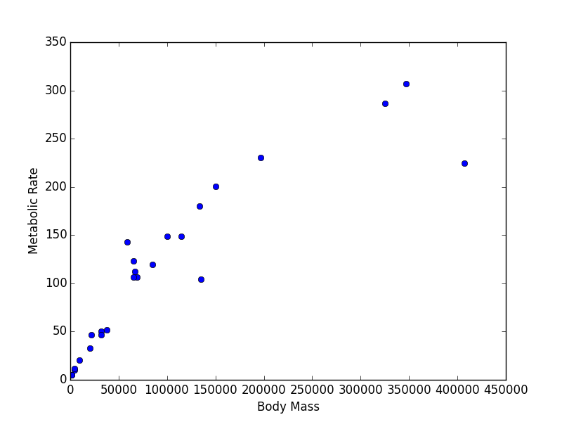
The relationship between the body size of an organism and its metabolic rate is one of the most well studied and still most controversial areas of organismal physiology. We want to graph this relationship in the Artiodactyla using a subset of data from a large compilation of body size data (Savage et al. 2004). You can copy and paste these two lists into your program:
body_mass = [32000, 37800, 347000, 4200, 196500, 100000, 4290,
32000, 65000, 69125, 9600, 133300, 150000, 407000, 115000, 67000,
325000, 21500, 58588, 65320, 85000, 135000, 20500, 1613, 1618]

metabolic_rate = [49.984, 51.981, 306.770, 10.075, 230.073,
148.949, 11.966, 46.414, 123.287, 106.663, 20.619, 180.150,
200.830, 224.779, 148.940, 112.430, 286.847, 46.347, 142.863,
106.670, 119.660, 104.150, 33.165, 4.900, 4.865]
Now make two plots with appropriate axis labels:
- A graph of body mass vs. metabolic rate
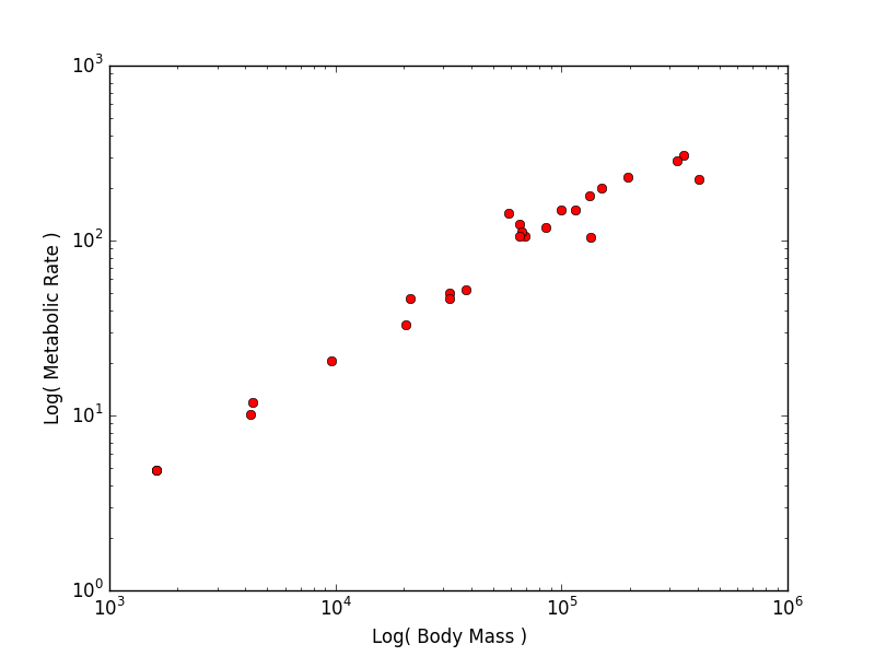
- A graph of log(body mass) vs. log(metabolic rate)
Think about what the shape of these graphs tells you about the form of the relationship between mass and metabolic rate.
Optional: If you like to make this a little more challenging (and see something really cool), try getting the raw data and selecting just the Artiodactyla data yourself. Unfortunately the raw data is trapped in a table that’s just part of the article webpage. Fortunately, Pandas will automatically read the tables out of a webpage for us using its
read_htmlmethod. So, you can just rundata = pd.read_html("http://onlinelibrary.wiley.com/doi/10.1111/j.0269-8463.2004.00856.x/full")and it will give us all of the tables from the web page, stored in a list. Pick the first table out of the list and you’ll be ready to get to work
NOTE: If you are using Enthought Canopy you will need a full Canopy license. Academics can get this for free at https://store.enthought.com/#canopy-academic. Then use the package manager to add
[click here for output] [click here for output]lxml.-- Adult vs Newborn Size 1 --
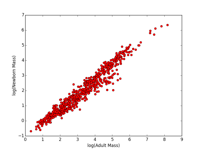
It makes sense that larger organisms have larger offspring, but what the mathematical form of this relationship should be is unclear. Let’s look at the problem empirically for mammals.
Download some mammal life history data from the web. You can do this either directly in the program using
urllibor download the file to your computer using your browser and import it from there.Import the data into a Pandas data frame. There are some extra blank lines at the end of this file, so get rid of them by using the optional
read_csv()argument,skip_footer=7.Missing data in this file is specified by -999 and -999.00. Tell Pandas that these are null values using the optional
read_csv()argument,na_values=['-999', '-999.00']. This will stop them from being plotted.- Graph adult mass vs. newborn mass. Label the axes.
- Graph the log (base 10) of adult mass vs. the log (base 10) of newborn mass. Label the axes.
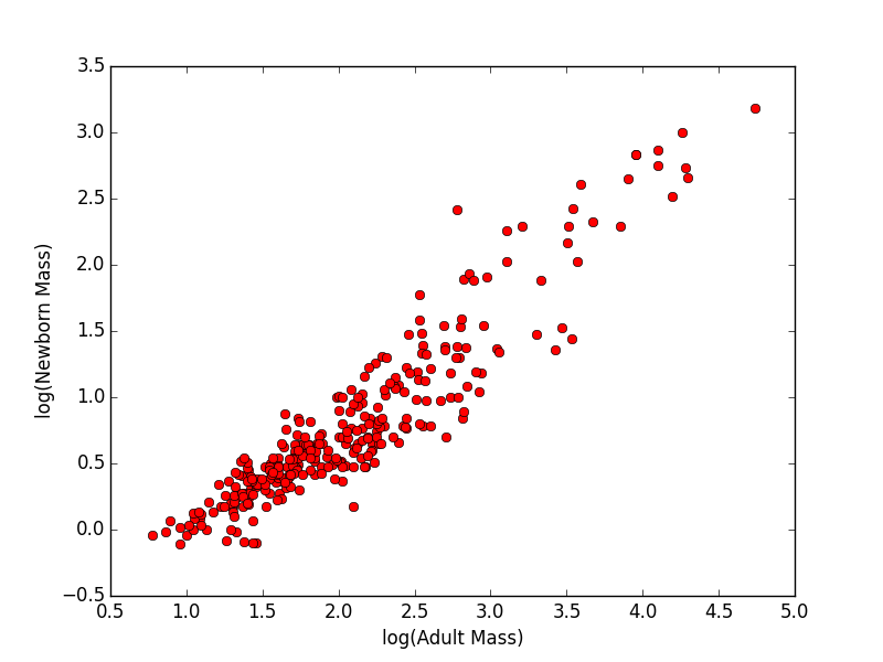
- For data where
orderisRodentia, graph the log (base 10) of adult mass vs. the log (base 10) of newborn mass. Label the axes.
-- Mammal Body Size 3 --
This is a follow up to Mammal Body Size 2.
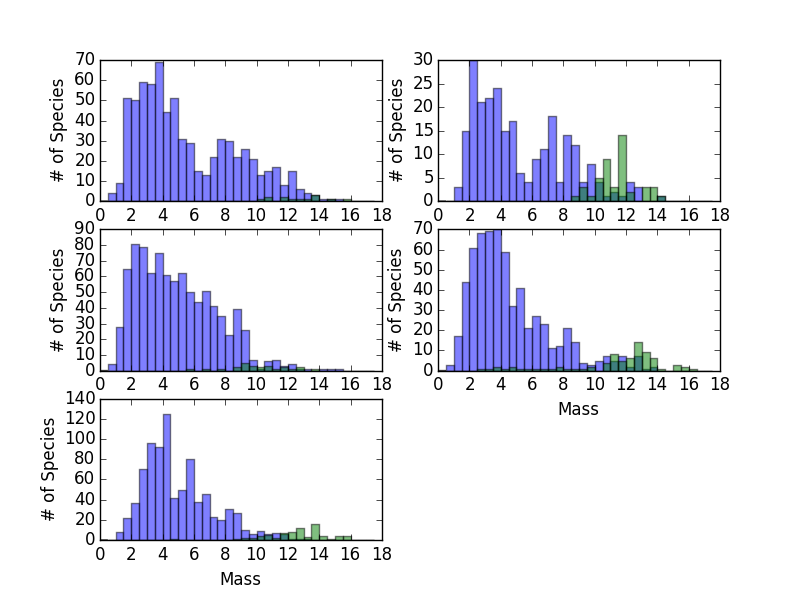
We have previously compared the average masses of extant and extinct species on different continents to try to understand whether size has an influence on extinction in mammals. Looking at the averages was a good start, but we really need to look at the full distributions of masses of the two groups to get the best picture of whether or not there was a major size bias in extinctions during the late Pleistocene. Make a graph with a subplot for each continent that you think is worth visualizing. Each subplot should contain two histograms that use the same bins to display the number of extinct and extant species. Use the log(mass) rather than the mass itself so that you can see the form of the distributions more clearly. Label the axes appropriately. The optional argument
alphawill allow you to make the histograms transparent, which will help with visualizing two histograms that overlap one another.There is a lot of work to do in this problem so make sure to break it down in to manageable pieces. Some logical chunks include:
- Make a single graph with the histograms for extinct and extant species. This might work well as its own function.
- Downloading/importing the data
- Breaking the data up into separate continents
- Breaking the data up into extinct and extant species
- Looping over the data to make one plot of each continent