
Learning Objectives
Following this assignment students should be able to:
- import, view properties, and plot a
raster- perform simple
rastermath- extract points from a
rasterusing a shapefile- evaluate a time series of
raster
Reading
-
Topics
raster- Raster math
- Plotting spatial images
- Shapefile import
- Integrate
rasterandvectordata
-
Readings
Lecture Notes
Exercises
-- Canopy Height from Space --
The National Ecological Observatory Network has invested in high-resolution airborne imaging of their field sites. Elevation models generated from LiDAR can be used to map the topography and vegetation structure at the sites. This data gets really powerful when you can compare ecological processes across sites. Download the elevation models for the Harvard Forest (
HARV) and San Joaquin Experimental Range (SJER) and the plot locations for each of these sites. Often, plots within a site are used as representative samples of the larger site and act as reference areas to obtain more detailed information and ensure accuracy of satellite imagery (i.e., ground truth).-
Create two Canopy Height Models using simple
rastermath (chm = dsm - dtm), one for theHARVsite (which was done during the lecture) and another for theSJERsite. -
Create plots and histograms of canopy heights for both of the sites on a single panel. To do so, type in the following line first to set up the panel:
par(mfrow = c(2, 2), mar = c(5, 4, 2, 2)). This specifies that there will be four figures on the same panel, and their margins. In the following lines, create the four plots usingplot()andhist(). If you run these five lines together, they should create a 4-figured panel. -
Add corresponding points from
plot_locationsfolder to each site plot. Don’t forget to use theadd = TRUEargument to add one plot on top of another. If points don’t show up, compare the crs of the canopy height model and the plot locations. -
Create a single dataframe with two columns, one of the maximum canopy heights for each point at the
HARVsite and one for theSJERpoints’ maximum canopy heights. When extracting the canopy height values, use a buffer of 10.
-
-- Phenology from Space --
The high-resolution images from Canopy Height from Space can be integrated with satellite imagery that is gathered more frequently. We will use data collected from MODIS. One common ecological process that can be observed from space is phenology (or seasonal patterns) of plants. Multi-band satellite imagery can be processed to provide a vegetation index of greenness called NDVI. NDVI values range from
-1.0to1.0, where negative values indicate clouds, snow, and water; bare soil returns values from0.1to0.2; and green vegetation returns values greater than0.3.Download HARV_NDVI and SJER_NDVI and place them in a folder with the NEON airborne data. The
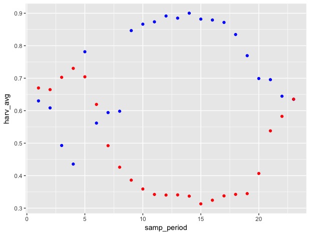
zipcontain folders with a year’s worth of NDVI sampling from MODIS. The files are in order (and named) by date and can be organized implicitly by sampling period for analysis.- Plot the whole-raster mean NDVI (
cellStats()) for Harvard Forest and SJER through time using different colors for the two sites. - Extract the NDVI values from all rasters for the
HARV_plotsandSJER_plotsinNEON-airborne/plot_locations. This results in a matrix with one column per raster and one row per point. To more easily work with this data, we want to have one column with the raster names and one column per point, which you can do by transposing the matrix with thet()function. Then make this into a dataframe and turn the rownames into a column. Do this for bothHARVandSJER.
- Plot the whole-raster mean NDVI (
-- Species Occurrences Elevation Histogram --
A colleague of yours is working on a project on deer mice (Peromyscus maniculatus) and is interested in what elevations these mice tend to occupy in the continental United States. You offer to help them out by getting some coordinates for specimens of this species and looking up the elevation of these coordinates.
-
Get deer mouse occurrences from GBIF, the Global Biodiversity Information Facility, using the
spoccR package, which is designed to retrieve species occurrence data from various openly available data resources. Use the following code to do so:mouse_df = occ(query = "Peromyscus maniculatus", from = "gbif") mouse_df = data.frame(mouse_df$gbif$data) -
With
dplyr, rename the second and third columns of this dataset tolongitudeandlatitude, and include only those specimens with abasisOfRecordthat isPRESERVED_SPECIMEN. -
The
rasterpackage comes with some datasets, including one of global elevations, that can be retrieved with thegetDatafunction as follows:elevation = getData("alt", country = "US") elevation = elevation[[1]] -
Turn the occurrences dataframe into a spatial dataframe, making sure that its projection matches that of the elevation dataset.
-
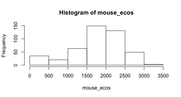
Extract the elevation values for all of the deer mouse occurrences and plot a histogram of them.
-
Write a function that creates a vector of elevation values for a given species name. This function should retrieve the data and put it into a dataframe, as in part 1. To limit how long this takes, add in the argument
limit = 50in theoccline. Then rename the latitude and longitude columns and remove NA rows from these columns using the following code:colnames(mouse_df)[2] <- "longitude" colnames(mouse_df)[3] <- "latitude" mouse_df = mouse_df %>% filter(!is.na(longitude) & !is.na(latitude))Turn the dataframe into a spatial object and extract the elevations for the points in the object. Test that your function works by putting in
"Peromyscus maniculatus"as the argument. -
Run this function on the following vector of mouse species names using either a loop to get a vector or an apply function to get a list of elevations for 50 occurrences of each of these 5 species.
mouse_species = c("Peromyscus maniculatus", "Peromyscus leucopus", "Peromyscus eremicus", "Peromyscus merriami", "Peromyscus boylii")
-