---
title: "Barnacle"
description: "final push"
categories: ["Transcriptomics"]
#citation:
date: 11-29-2025
image: http://gannet.fish.washington.edu/seashell/snaps/Monosnap_Image_2025-11-30_15-34-25.png # finding a good image
author:
- name: Steven Roberts
url:
orcid: 0000-0001-8302-1138
affiliation: Professor, UW - School of Aquatic and Fishery Sciences
affiliation-url: https://robertslab.info
#url: # self-defined
draft: false # setting this to `true` will prevent your post from appearing on your listing page until you're ready!
format:
html:
toc: true # ← enable TOC
toc-location: left # or: right, body
toc-depth: 3 # how many heading levels to show
code-fold: FALSE
code-tools: true
code-copy: true
highlight-style: github
code-overflow: wrap
#runtime: shiny
---
## Trying to build alternative tensor
``` python
#!/usr/bin/env python3
"""
Alternative tensor construction: (genes × timepoints × samples)
Each sample becomes a separate slice instead of grouping by species.
"""
import argparse
import json
import os
from datetime import datetime
from typing import Dict, List, Tuple

import numpy as np
import pandas as pd
import matplotlib.pyplot as plt

from barnacle.decomposition import SparseCP


def read_normalized_csv(path: str) -> pd.DataFrame:
    df = pd.read_csv(path)
    if 'group_id' not in df.columns:
        raise ValueError(f"Expected 'group_id' column in {path}")
    df = df.set_index('group_id')
    return df


def parse_sample_timepoint(column_name: str) -> Tuple[str, str, int]:
    tp_index = column_name.rfind('-TP')
    if tp_index == -1:
        raise ValueError(f"Expected TP# token at end of column: {column_name}")

    time_token = column_name[tp_index + 1:]
    if not time_token.startswith('TP'):
        raise ValueError(f"Expected TP# token at end of column: {column_name}")
    try:
        tp = int(time_token.replace('TP', ''))
    except Exception as exc:
        raise ValueError(f"Failed to parse timepoint from {column_name}") from exc

    sample_id = column_name[:tp_index]
    sample_prefix = sample_id.split('-')[0]
    species_map = {'ACR': 'apul', 'POR': 'peve', 'POC': 'ptua'}
    if sample_prefix not in species_map:
        raise ValueError(f"Unknown species prefix in column: {column_name}")

    species = species_map[sample_prefix]
    return species, sample_id, tp


def build_tensor_by_sample(
    df: pd.DataFrame,
    expected_timepoints: List[int],
) -> Tuple[np.ndarray, List[str], Dict[int, Dict[str, str]], List[str]]:
    """
    Build tensor with shape (genes, timepoints, samples).
    Each unique sample becomes a slice, with timepoints as rows.
    """
    common_genes = sorted(list(df.index))

    # Collect all unique samples across all species
    sample_data = {}  # {sample_id: {species: str, columns: {tp: col_name}}}

    for col in df.columns:
        try:
            species, sample_id, tp = parse_sample_timepoint(col)
            if tp in expected_timepoints:
                if sample_id not in sample_data:
                    sample_data[sample_id] = {
                        'species': species,
                        'columns': {}
                    }
                sample_data[sample_id]['columns'][tp] = col
        except ValueError:
            continue

    # Sort samples by species, then by sample_id
    sorted_samples = sorted(
        sample_data.keys(),
        key=lambda sid: (sample_data[sid]['species'], sid)
    )

    # Build sample labels and metadata
    sample_labels: List[str] = []
    sample_metadata: Dict[int, Dict[str, str]] = {}

    for idx, sample_id in enumerate(sorted_samples):
        species = sample_data[sample_id]['species']
        sample_labels.append(f"{species}_{sample_id}")
        sample_metadata[idx] = {
            'species': species,
            'sample_id': sample_id,
        }

    n_genes = len(common_genes)
    n_time = len(expected_timepoints)
    n_samples = len(sorted_samples)

    if n_samples == 0:
        raise ValueError("No samples with valid timepoints found")

    # Tensor shape: (genes, timepoints, samples)
    tensor = np.empty((n_genes, n_time, n_samples), dtype=float)
    tensor[:] = np.nan

    # Fill tensor
    for s_idx, sample_id in enumerate(sorted_samples):
        columns = sample_data[sample_id]['columns']
        for t_idx, tp in enumerate(expected_timepoints):
            col = columns.get(tp)
            if col is None:
                continue
            values = df.loc[common_genes, col].to_numpy(dtype=float)
            tensor[:, t_idx, s_idx] = values

    # Replace NaNs with zeros
    tensor = np.nan_to_num(tensor, nan=0.0)
    return tensor, sample_labels, sample_metadata, common_genes


def run_sparse_cp(
    tensor: np.ndarray,
    rank: int,
    lambda_gene: float,
    lambda_time: float,
    lambda_sample: float,
    max_iter: int,
    tol: float,
    seed: int,
):
    """
    Note: lambda order now matches tensor dimensions: [gene, time, sample]
    """
    model = SparseCP(
        rank=rank,
        lambdas=[lambda_gene, lambda_time, lambda_sample],
        nonneg_modes=[0],
        n_initializations=3,
        random_state=seed,
        n_iter_max=max_iter,
        tol=tol,
    )
    decomposition = model.fit_transform(tensor, verbose=1)
    return model, decomposition


def save_outputs(
    output_dir: str,
    tensor: np.ndarray,
    sample_labels: List[str],
    sample_metadata: Dict[int, Dict[str, str]],
    genes: List[str],
    model,
    decomposition,
):
    os.makedirs(output_dir, exist_ok=True)
    factors_dir = os.path.join(output_dir, 'barnacle_factors')
    figs_dir = os.path.join(output_dir, 'figures')
    os.makedirs(factors_dir, exist_ok=True)
    os.makedirs(figs_dir, exist_ok=True)

    np.save(os.path.join(output_dir, 'multiomics_tensor.npy'), tensor)

    # Extract factors: order is [genes, timepoints, samples]
    gene_factors = pd.DataFrame(decomposition.factors[0], index=genes)
    time_factors = pd.DataFrame(decomposition.factors[1],
                               index=[f'TP{t}' for t in range(1, tensor.shape[1] + 1)])
    sample_factors = pd.DataFrame(decomposition.factors[2], index=sample_labels)

    gene_factors.to_csv(os.path.join(factors_dir, 'gene_factors.csv'))
    time_factors.to_csv(os.path.join(factors_dir, 'time_factors.csv'))
    sample_factors.to_csv(os.path.join(factors_dir, 'sample_factors.csv'))

    # Compute component weights
    weights_attr = getattr(decomposition, 'weights', None)
    if weights_attr is not None:
        weights = np.asarray(weights_attr).astype(float).ravel()
        if np.allclose(weights, weights[0]) if len(weights) > 0 else True:
            weights = None
    else:
        weights = None

    if weights is None:
        gene_norms = np.linalg.norm(gene_factors.values, axis=0)
        time_norms = np.linalg.norm(time_factors.values, axis=0)
        sample_norms = np.linalg.norm(sample_factors.values, axis=0)
        weights = gene_norms * time_norms * sample_norms

    pd.DataFrame({'weight': weights}).to_csv(
        os.path.join(factors_dir, 'component_weights.csv'), index=False)

    # Sample mapping
    mapping_rows = []
    for idx, label in enumerate(sample_labels):
        mapping_rows.append({
            'sample_index': idx,
            'label': label,
            'species': sample_metadata[idx]['species'],
            'sample_id': sample_metadata[idx]['sample_id'],
        })
    pd.DataFrame(mapping_rows).to_csv(
        os.path.join(factors_dir, 'sample_mapping.csv'), index=False)

    # Metadata
    raw_loss = getattr(model, 'loss_', None)
    if raw_loss is None:
        final_loss = None
    else:
        try:
            if isinstance(raw_loss, (list, tuple, np.ndarray)) and len(raw_loss) > 0:
                final_loss = float(raw_loss[-1])
            else:
                final_loss = float(raw_loss)
        except Exception:
            final_loss = None

    metadata = {
        'timestamp': datetime.utcnow().isoformat() + 'Z',
        'tensor_shape': list(map(int, tensor.shape)),
        'tensor_structure': '(genes, timepoints, samples)',
        'n_components': int(gene_factors.shape[1]),
        'model_converged': bool(getattr(model, 'converged_', False)),
        'final_loss': final_loss,
    }
    with open(os.path.join(factors_dir, 'metadata.json'), 'w') as fh:
        json.dump(metadata, fh, indent=2)

    # Figures
    plt.figure(figsize=(6, 4))
    plt.bar(np.arange(len(weights)), weights)
    plt.xlabel('Component')
    plt.ylabel('Weight')
    plt.title('Component Weights')
    plt.tight_layout()
    plt.savefig(os.path.join(figs_dir, 'component_weights.png'), dpi=200)
    plt.close()

    # Time loadings across components
    plt.figure(figsize=(7, 4))
    for k in range(time_factors.shape[1]):
        plt.plot(range(1, time_factors.shape[0] + 1),
                time_factors.iloc[:, k], marker='o', label=f'C{k+1}')
    plt.xticks(range(1, time_factors.shape[0] + 1))
    plt.xlabel('Timepoint')
    plt.ylabel('Loading')
    plt.title('Time Loadings by Component')
    plt.legend(ncols=2, fontsize=8)
    plt.tight_layout()
    plt.savefig(os.path.join(figs_dir, 'time_loadings.png'), dpi=200)
    plt.close()

    # Sample loadings colored by species
    fig, ax = plt.subplots(figsize=(10, 6))
    species_colors = {'apul': 'C0', 'peve': 'C1', 'ptua': 'C2'}

    for k in range(sample_factors.shape[1]):
        for idx, label in enumerate(sample_labels):
            species = sample_metadata[idx]['species']
            ax.scatter(k, sample_factors.iloc[idx, k],
                      c=species_colors[species], alpha=0.6, s=50)

    ax.set_xlabel('Component')
    ax.set_ylabel('Sample Loading')
    ax.set_title('Sample Loadings by Component and Species')

    # Legend
    from matplotlib.patches import Patch
    legend_elements = [Patch(facecolor=species_colors[sp], label=sp)
                      for sp in ['apul', 'peve', 'ptua']]
    ax.legend(handles=legend_elements)
    plt.tight_layout()
    plt.savefig(os.path.join(figs_dir, 'sample_loadings.png'), dpi=200)
    plt.close()


def main() -> None:
    parser = argparse.ArgumentParser(
        description='Build tensor (genes × timepoints × samples) and run Barnacle SparseCP')
    parser.add_argument('--input-file', required=True,
                       help='Path to merged vst_counts_matrix.csv file')
    parser.add_argument('--output-dir', required=True,
                       help='Output directory for results')
    parser.add_argument('--rank', type=int, default=5)
    parser.add_argument('--lambda-gene', type=float, default=0.1)
    parser.add_argument('--lambda-time', type=float, default=0.05)
    parser.add_argument('--lambda-sample', type=float, default=0.1)
    parser.add_argument('--max-iter', type=int, default=1000)
    parser.add_argument('--tol', type=float, default=1e-5)
    parser.add_argument('--seed', type=int, default=42)
    args = parser.parse_args()

    if not os.path.exists(args.input_file):
        raise FileNotFoundError(f"Input file not found: {args.input_file}")

    df = read_normalized_csv(args.input_file)
    tensor, sample_labels, sample_metadata, genes = build_tensor_by_sample(
        df, expected_timepoints=[1, 2, 3, 4])

    print(f"\nTensor shape: {tensor.shape}")
    print(f"  Genes: {tensor.shape[0]}")
    print(f"  Timepoints: {tensor.shape[1]}")
    print(f"  Samples: {tensor.shape[2]}")

    model, decomposition = run_sparse_cp(
        tensor=tensor,
        rank=args.rank,
        lambda_gene=args.lambda_gene,
        lambda_time=args.lambda_time,
        lambda_sample=args.lambda_sample,
        max_iter=args.max_iter,
        tol=args.tol,
        seed=args.seed,
    )

    save_outputs(args.output_dir, tensor, sample_labels, sample_metadata,
                genes, model, decomposition)


if __name__ == '__main__':
    main()
```
### Output
```{r}
library(readr)
library(pheatmap)
library(tidyverse)
```
```{r}
gene_csv <-read.csv("https://gannet.fish.washington.edu/v1_web/owlshell/bu-github/timeseries_molecular/M-multi-species/output/50-tensor-alternative/barnacle_factors/gene_factors.csv",
               check.names = FALSE)

# Replace column names
colnames(gene_csv) <- c("OG_ID", paste0("Component_", 1:(ncol(gene_csv)-1)))
```
```{r}
time_csv <-read.csv("https://gannet.fish.washington.edu/v1_web/owlshell/bu-github/timeseries_molecular/M-multi-species/output/50-tensor-alternative/barnacle_factors/time_factors.csv",
               check.names = FALSE)

# Replace column names
colnames(time_csv) <- c("Time_ID", paste0("Component_", 1:(ncol(time_csv)-1)))
```
```{r}
# Path to your CSV file
sample_csv <- read.csv("https://gannet.fish.washington.edu/v1_web/owlshell/bu-github/timeseries_molecular/M-multi-species/output/50-tensor-alternative/barnacle_factors/sample_factors.csv",
               check.names = FALSE)

# Replace column names
colnames(sample_csv) <- c("Sample", paste0("Component_", 1:(ncol(sample_csv)-1)))
```
```{r}
# Load required libraries
library(readr)
library(pheatmap)


# Make the first column row names
df_mat <- sample_csv |>
  column_to_rownames(var = colnames(sample_csv)[1]) |>
  as.matrix()

# Optional: scale rows or columns for better contrast
df_scaled <- scale(df_mat)

# Plot heatmap
pheatmap(df_scaled,
         color = colorRampPalette(c("navy","white","firebrick3"))(100),
         clustering_method = "ward.D2",
         show_rownames = TRUE,
         show_colnames = TRUE,
         main = "Heatmap of Samples vs Features")
```
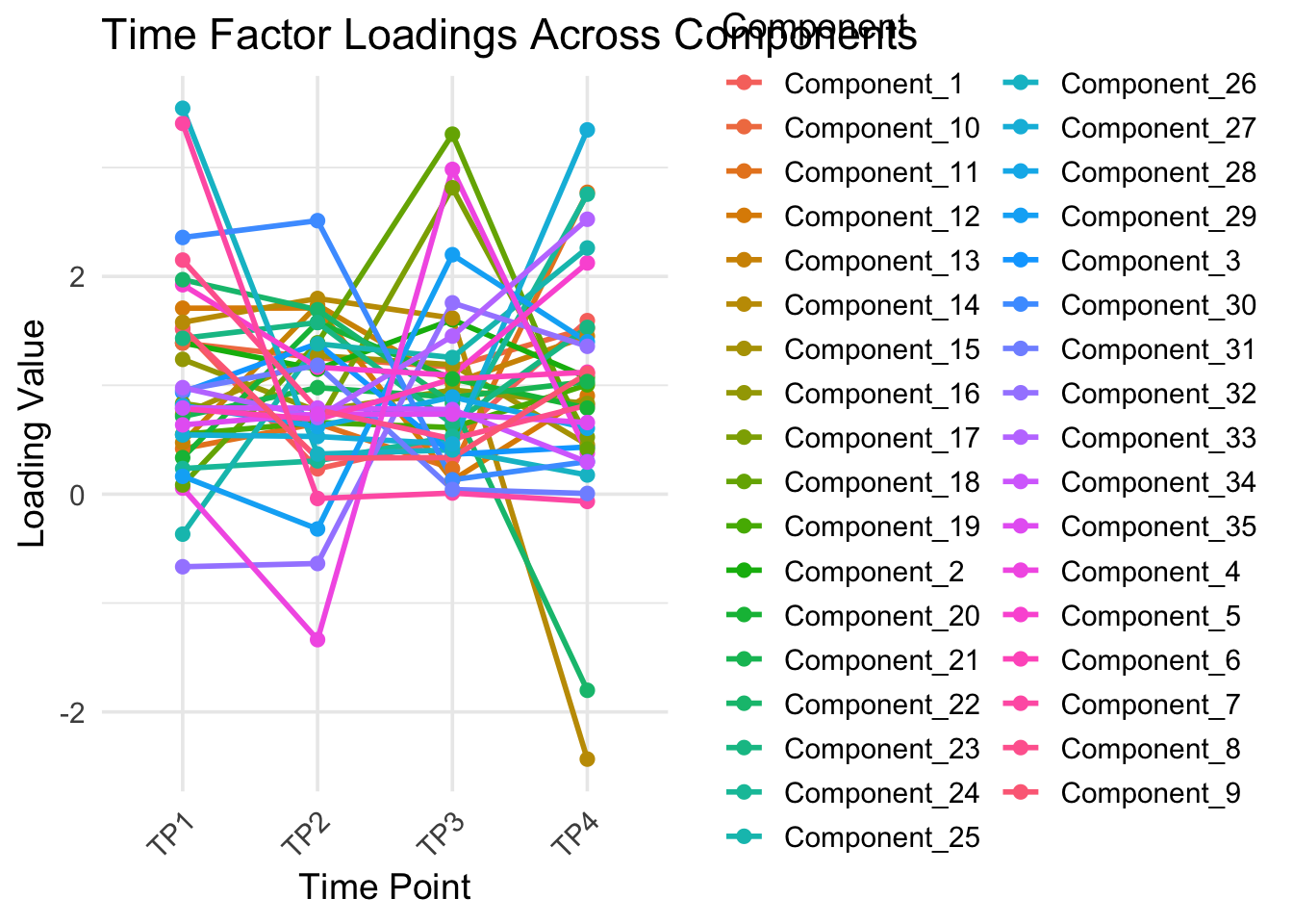
```{r}
library(tidyverse)

# Pivot to long format for plotting
df_long <- time_csv %>%
  pivot_longer(
    cols = starts_with("Component_"),
    names_to = "Component",
    values_to = "Value"
  )

# Line plot
ggplot(df_long, aes(x = Time_ID, y = Value, group = Component, color = Component)) +
  geom_line(linewidth = 1) +
  geom_point(size = 2) +
  theme_minimal(base_size = 14) +
  theme(
    axis.text.x = element_text(angle = 45, hjust = 1),
    legend.position = "right"
  ) +
  labs(
    title = "Time Factor Loadings Across Components",
    x = "Time Point",
    y = "Loading Value"
  )
```
```{r}
library(tidyverse)


# Compute variance of each component across timepoints
var_components <- time_csv %>%
  pivot_longer(cols = starts_with("Component_"),
               names_to = "Component",
               values_to = "Value") %>%
  group_by(Component) %>%
  summarise(Variance = var(Value, na.rm = TRUE)) %>%
  arrange(desc(Variance))

# Select top 10 most variable components
top10_components <- var_components %>% slice_max(Variance, n = 10) %>% pull(Component)

# Prepare data for plotting
time_csv_long <- time_csv %>%
  pivot_longer(cols = starts_with("Component_"),
               names_to = "Component",
               values_to = "Value") %>%
  filter(Component %in% top10_components)

# Line plot
ggplot(time_csv_long, aes(x = Time_ID, y = Value, group = Component, color = Component)) +
  geom_line(linewidth = 1.2) +
  geom_point(size = 2) +
  theme_minimal(base_size = 14) +
  theme(axis.text.x = element_text(angle = 45, hjust = 1)) +
  labs(
    title = "Top 10 Most Variable Components Across Timepoints",
    x = "Time Point",
    y = "Component Value"
  )
```
```{r}
library(tidyverse)


# ---- USER INPUT ----
# Pick the component you want to plot (e.g., "Component_5")
selected_component <- "Component_5"
# ---------------------


# Convert to long format
df_long <- time_csv %>%
  pivot_longer(
    cols = starts_with("Component_"),
    names_to = "Component",
    values_to = "Value"
  )

# Check that the chosen component exists
if (!(selected_component %in% unique(df_long$Component))) {
  stop(paste("Component", selected_component, "not found in data!"))
}

# Filter for the selected component
df_sel <- df_long %>% filter(Component == selected_component)

# Plot single component across timepoints
ggplot(df_sel, aes(x = Time_ID, y = Value, group = 1)) +
  geom_line(linewidth = 1.2, color = "steelblue") +
  geom_point(size = 3, color = "firebrick") +
  theme_minimal(base_size = 14) +
  theme(axis.text.x = element_text(angle = 45, hjust = 1)) +
  labs(
    title = paste0(selected_component, " Across Timepoints"),
    x = "Time Point",
    y = "Loading Value"
  )
```
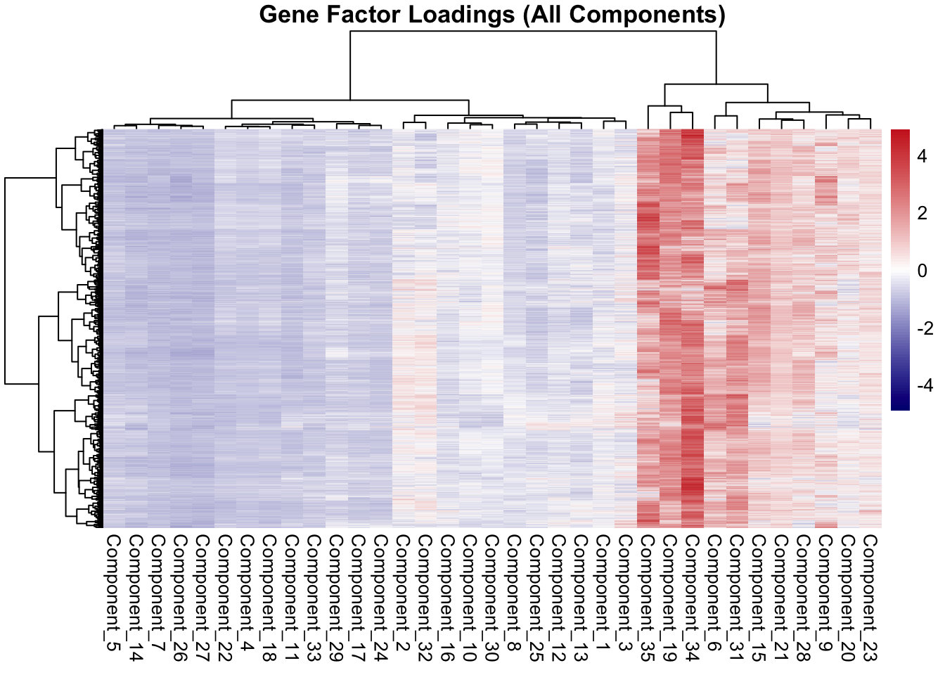
```{r}
library(tidyverse)
library(pheatmap)


# Convert to matrix (remove OG_ID column)
mat <- gene_csv %>%
  column_to_rownames(var = "OG_ID") %>%
  as.matrix()


# Optional: scale rows (genes) so colors represent relative loadings per gene
pheatmap(
  mat,
  scale = "row",
  color = colorRampPalette(c("navy", "white", "firebrick3"))(100),
  clustering_method = "ward.D2",
  show_rownames = FALSE,
  main = "Gene Factor Loadings (All Components)"
)
```
```{r}
library(tidyverse)
library(pheatmap)


# Convert to numeric matrix
mat <- gene_csv %>%
  column_to_rownames(var = "OG_ID") %>%
  as.matrix()

# Heatmap of actual (unscaled) values
pheatmap(
  mat,
  scale = "none",  # do not scale
  color = colorRampPalette(c("navy", "white", "firebrick3"))(200),
  clustering_method = "ward.D2",
  show_rownames = FALSE,
  main = "Gene Factor Loadings (Actual Values)"
)
```
## More lamda testing
``` bash
LAMBDAS_GENE="0.00 0.1 0.2 0.4 0.8 1.0 10 40 100 1000"
LAMBDA_SAMPLE=0.1
LAMBDA_TIME=0.05
RANK=35

mkdir -p ../output/40-rank35-optimization

OUTDIR_BASE=../output/40-rank35-optimization

for LG in $LAMBDAS_GENE; do
  OUTDIR=${OUTDIR_BASE}/lambda_gene_${LG}
  mkdir -p "$OUTDIR"

  uv run python ../scripts/14.1-barnacle/build_tensor_and_run.py \
    --input-file ../output/14-pca-orthologs/vst_counts_matrix.csv \
    --output-dir "$OUTDIR" \
    --rank $RANK \
    --lambda-gene $LG \
    --lambda-sample $LAMBDA_SAMPLE \
    --lambda-time $LAMBDA_TIME \
    --max-iter 1000 \
    --tol 1e-5 \
    --seed 92
done
```
```{r, echo=TRUE, warning=FALSE, message=FALSE}
library(tidyverse)

# ---------------------------------------------------------
# SETTINGS
# ---------------------------------------------------------

base_url <- "https://gannet.fish.washington.edu/v1_web/owlshell/bu-github/timeseries_molecular/M-multi-species/output/40-rank35-optimization"

lambda_vals <- c("0.00","0.1","0.2","0.4","0.8","1.0","10","40","100","1000")

# ---------------------------------------------------------
# FUNCTION: read gene_factors.csv AND FIX HEADER
# ---------------------------------------------------------
read_gene_factors <- function(lambda) {
  url <- sprintf("%s/lambda_gene_%s/barnacle_factors/gene_factors.csv",
                 base_url, lambda)

  message("Reading: ", url)
  df <- read_csv(url, show_col_types = FALSE)

  # Fix the shifted header here
  # First column should be "gene", others "comp1..compN"
  colnames(df) <- c("gene", paste0("comp", 1:(ncol(df)-1)))

  df$lambda_gene <- lambda
  df
}

# ---------------------------------------------------------
# READ ALL RUNS
# ---------------------------------------------------------
all_factors <- map_df(lambda_vals, read_gene_factors)

# ---------------------------------------------------------
# LONG FORMAT FOR ANALYSIS
# ---------------------------------------------------------
factor_long <- all_factors %>%
  pivot_longer(
    cols = starts_with("comp"),
    names_to = "component",
    values_to = "loading"
  )
```
```{r}
sparsity_tbl <- factor_long %>%
  group_by(lambda_gene) %>%
  summarize(
    n_values = n(),
    n_zero = sum(loading == 0 | abs(loading) < 1e-12),
    sparsity = n_zero / n_values
  )

sparsity_tbl
```
```{r}
gene_component_counts <- factor_long %>%
  filter(loading > 0) %>%
  group_by(lambda_gene, gene) %>%
  summarize(
    n_components = n_distinct(component),
    .groups = "drop"
  )
```
```{r}
multi_component_summary <- gene_component_counts %>%
  group_by(lambda_gene, n_components) %>%
  summarize(n_genes = n(), .groups = "drop")

multi_component_summary
```
```{r}
summary_tbl <- sparsity_tbl %>%
  left_join(
    gene_component_counts %>%
      group_by(lambda_gene) %>%
      summarize(
        mean_components = mean(n_components),
        frac_multi = mean(n_components > 1),
        .groups = "drop"
      ),
    by = "lambda_gene"
  )

summary_tbl
```
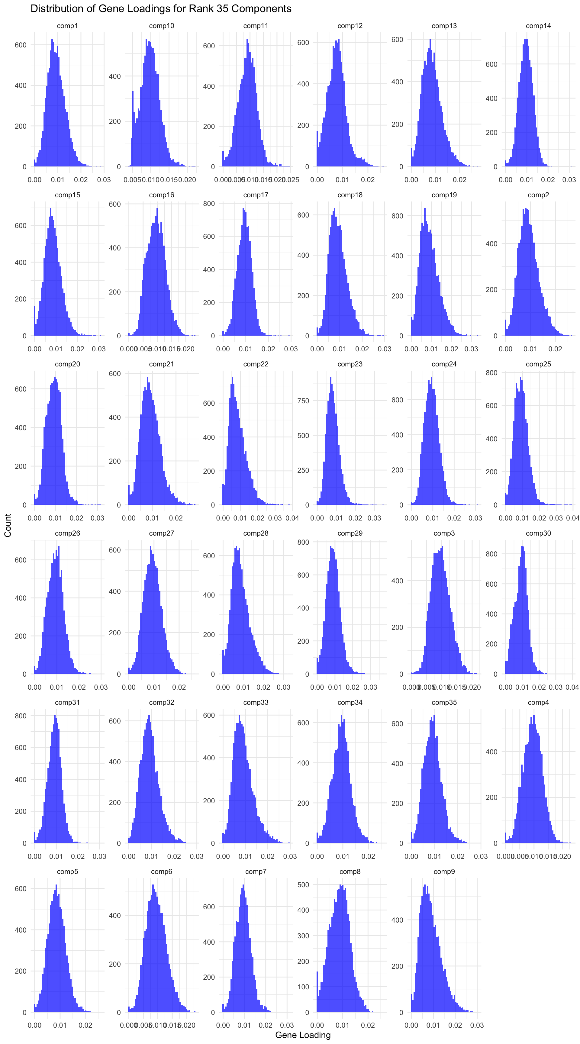
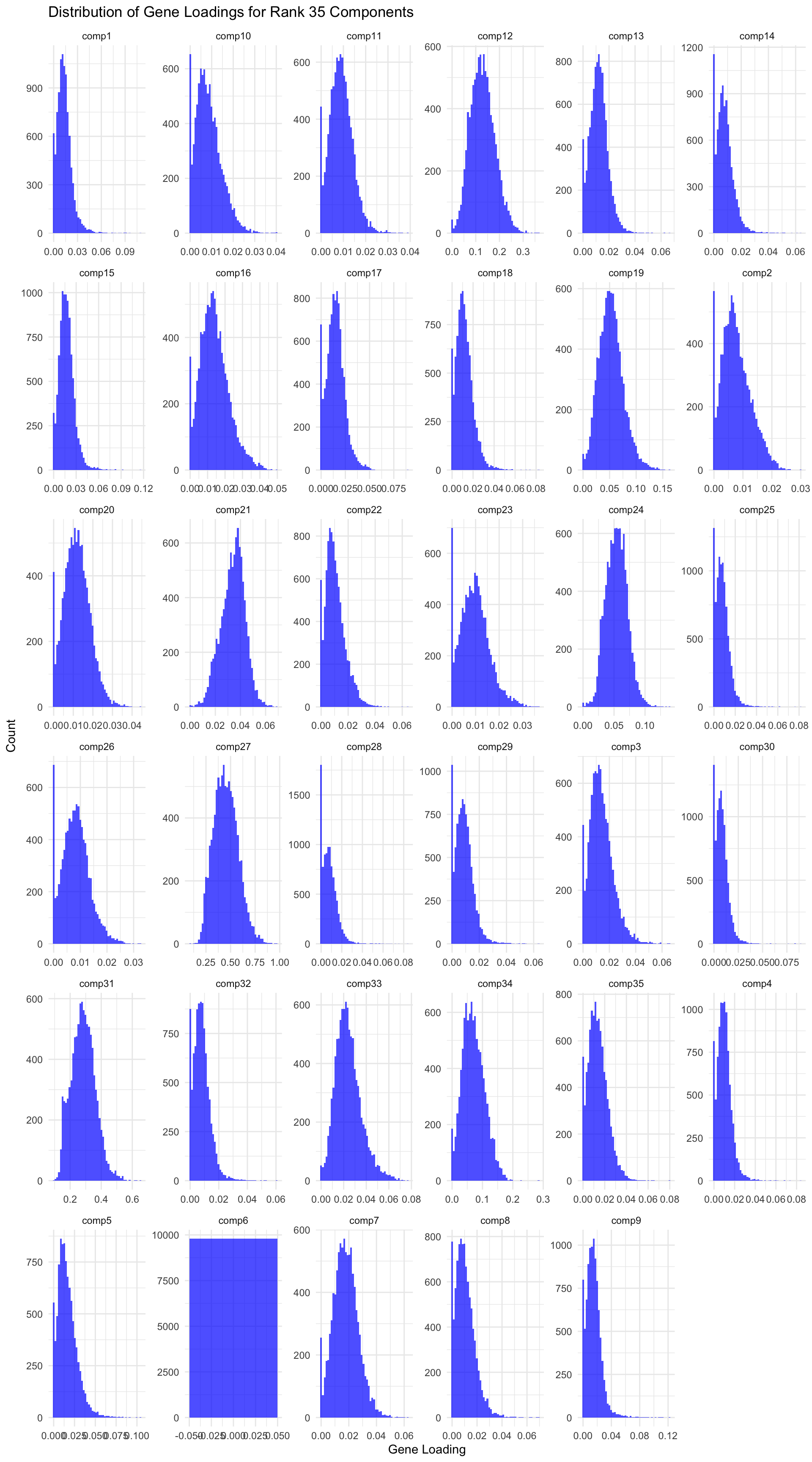
```{r, echo=TRUE, warning=FALSE, message=FALSE, fig.width=10, fig.height=18}
  # Load data
  gene_factors <- read_csv("https://gannet.fish.washington.edu/v1_web/owlshell/bu-github/timeseries_molecular/M-multi-species/output/40-rank35-optimization/lambda_gene_0.00/barnacle_factors/gene_factors.csv")


#edit so columns names are shifted 1 to the left
  colnames(gene_factors) <- c("gene", paste0("comp", 1:(ncol(gene_factors)-1)))

#code to create histogram of gene_factors:

  library(ggplot2)
  library(tidyr)

  # Reshape data to long format
  gene_factors_long <- gene_factors %>%
    pivot_longer(cols = -1, names_to = "component", values_to = "loading")

  # Plot histogram
  ggplot(gene_factors_long, aes(x = loading)) +
    geom_histogram(bins = 50, fill = "blue", alpha = 0.7) +
    facet_wrap(~ component, scales = "free") +
    theme_minimal() +
    labs(title = "Distribution of Gene Loadings for Rank 35 Components",
         x = "Gene Loading",
         y = "Count")
```
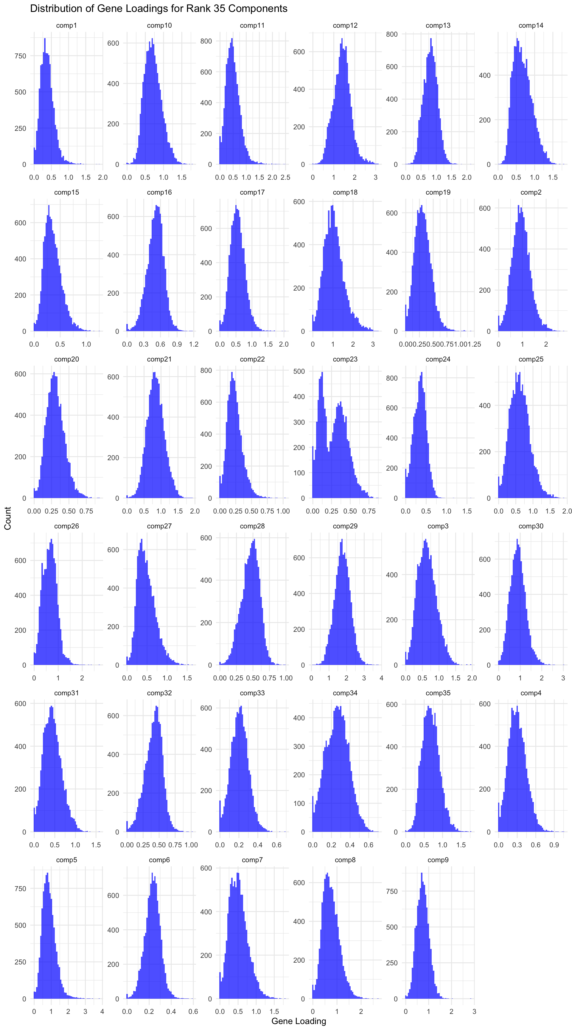
```{r, echo=TRUE, warning=FALSE, message=FALSE, fig.width=10, fig.height=18}
  # Load data
  gene_factors <- read_csv("https://gannet.fish.washington.edu/v1_web/owlshell/bu-github/timeseries_molecular/M-multi-species/output/40-rank35-optimization/lambda_gene_0.1/barnacle_factors/gene_factors.csv")


#edit so columns names are shifted 1 to the left
  colnames(gene_factors) <- c("gene", paste0("comp", 1:(ncol(gene_factors)-1)))

#code to create histogram of gene_factors:

  library(ggplot2)
  library(tidyr)

  # Reshape data to long format
  gene_factors_long <- gene_factors %>%
    pivot_longer(cols = -1, names_to = "component", values_to = "loading")

  # Plot histogram
  ggplot(gene_factors_long, aes(x = loading)) +
    geom_histogram(bins = 50, fill = "blue", alpha = 0.7) +
    facet_wrap(~ component, scales = "free") +
    theme_minimal() +
    labs(title = "Distribution of Gene Loadings for Rank 35 Components",
         x = "Gene Loading",
         y = "Count")
```
```{r, echo=TRUE, warning=FALSE, message=FALSE, fig.width=10, fig.height=18}
  # Load data
  gene_factors <- read_csv("https://gannet.fish.washington.edu/v1_web/owlshell/bu-github/timeseries_molecular/M-multi-species/output/40-rank35-optimization/lambda_gene_0.2/barnacle_factors/gene_factors.csv")


#edit so columns names are shifted 1 to the left
  colnames(gene_factors) <- c("gene", paste0("comp", 1:(ncol(gene_factors)-1)))

#code to create histogram of gene_factors:

  library(ggplot2)
  library(tidyr)

  # Reshape data to long format
  gene_factors_long <- gene_factors %>%
    pivot_longer(cols = -1, names_to = "component", values_to = "loading")

  # Plot histogram
  ggplot(gene_factors_long, aes(x = loading)) +
    geom_histogram(bins = 50, fill = "blue", alpha = 0.7) +
    facet_wrap(~ component, scales = "free") +
    theme_minimal() +
    labs(title = "Distribution of Gene Loadings for Rank 35 Components",
         x = "Gene Loading",
         y = "Count")
```
```{r, echo=TRUE, warning=FALSE, message=FALSE, fig.width=10, fig.height=18}
  # Load data
  gene_factors <- read_csv("https://gannet.fish.washington.edu/v1_web/owlshell/bu-github/timeseries_molecular/M-multi-species/output/40-rank35-optimization/lambda_gene_0.4/barnacle_factors/gene_factors.csv")


#edit so columns names are shifted 1 to the left
  colnames(gene_factors) <- c("gene", paste0("comp", 1:(ncol(gene_factors)-1)))

#code to create histogram of gene_factors:

  library(ggplot2)
  library(tidyr)

  # Reshape data to long format
  gene_factors_long <- gene_factors %>%
    pivot_longer(cols = -1, names_to = "component", values_to = "loading")

  # Plot histogram
  ggplot(gene_factors_long, aes(x = loading)) +
    geom_histogram(bins = 50, fill = "blue", alpha = 0.7) +
    facet_wrap(~ component, scales = "free") +
    theme_minimal() +
    labs(title = "Distribution of Gene Loadings for Rank 35 Components",
         x = "Gene Loading",
         y = "Count")
```
```{r, echo=TRUE, warning=FALSE, message=FALSE, fig.width=10, fig.height=18}
  # Load data
  gene_factors <- read_csv("https://gannet.fish.washington.edu/v1_web/owlshell/bu-github/timeseries_molecular/M-multi-species/output/40-rank35-optimization/lambda_gene_0.8/barnacle_factors/gene_factors.csv")


#edit so columns names are shifted 1 to the left
  colnames(gene_factors) <- c("gene", paste0("comp", 1:(ncol(gene_factors)-1)))

#code to create histogram of gene_factors:

  library(ggplot2)
  library(tidyr)

  # Reshape data to long format
  gene_factors_long <- gene_factors %>%
    pivot_longer(cols = -1, names_to = "component", values_to = "loading")

  # Plot histogram
  ggplot(gene_factors_long, aes(x = loading)) +
    geom_histogram(bins = 50, fill = "blue", alpha = 0.7) +
    facet_wrap(~ component, scales = "free") +
    theme_minimal() +
    labs(title = "Distribution of Gene Loadings for Rank 35 Components",
         x = "Gene Loading",
         y = "Count")
```
```{r, echo=TRUE, warning=FALSE, message=FALSE, fig.width=10, fig.height=18}
  # Load data
  gene_factors <- read_csv("https://gannet.fish.washington.edu/v1_web/owlshell/bu-github/timeseries_molecular/M-multi-species/output/40-rank35-optimization/lambda_gene_1.0/barnacle_factors/gene_factors.csv")


#edit so columns names are shifted 1 to the left
  colnames(gene_factors) <- c("gene", paste0("comp", 1:(ncol(gene_factors)-1)))

#code to create histogram of gene_factors:

  library(ggplot2)
  library(tidyr)

  # Reshape data to long format
  gene_factors_long <- gene_factors %>%
    pivot_longer(cols = -1, names_to = "component", values_to = "loading")

  # Plot histogram
  ggplot(gene_factors_long, aes(x = loading)) +
    geom_histogram(bins = 50, fill = "blue", alpha = 0.7) +
    facet_wrap(~ component, scales = "free") +
    theme_minimal() +
    labs(title = "Distribution of Gene Loadings for Rank 35 Components",
         x = "Gene Loading",
         y = "Count")
```
```{r, echo=TRUE, warning=FALSE, message=FALSE, fig.width=10, fig.height=18}
  # Load data
  gene_factors <- read_csv("https://gannet.fish.washington.edu/v1_web/owlshell/bu-github/timeseries_molecular/M-multi-species/output/40-rank35-optimization/lambda_gene_10/barnacle_factors/gene_factors.csv")


#edit so columns names are shifted 1 to the left
  colnames(gene_factors) <- c("gene", paste0("comp", 1:(ncol(gene_factors)-1)))

#code to create histogram of gene_factors:

  library(ggplot2)
  library(tidyr)

  # Reshape data to long format
  gene_factors_long <- gene_factors %>%
    pivot_longer(cols = -1, names_to = "component", values_to = "loading")

  # Plot histogram
  ggplot(gene_factors_long, aes(x = loading)) +
    geom_histogram(bins = 50, fill = "blue", alpha = 0.7) +
    facet_wrap(~ component, scales = "free") +
    theme_minimal() +
    labs(title = "Distribution of Gene Loadings for Rank 35 Components",
         x = "Gene Loading",
         y = "Count")
```
```{r, echo=TRUE, warning=FALSE, message=FALSE, fig.width=10, fig.height=18}
  # Load data
  gene_factors <- read_csv("https://gannet.fish.washington.edu/v1_web/owlshell/bu-github/timeseries_molecular/M-multi-species/output/40-rank35-optimization/lambda_gene_40/barnacle_factors/gene_factors.csv")


#edit so columns names are shifted 1 to the left
  colnames(gene_factors) <- c("gene", paste0("comp", 1:(ncol(gene_factors)-1)))

#code to create histogram of gene_factors:

  library(ggplot2)
  library(tidyr)

  # Reshape data to long format
  gene_factors_long <- gene_factors %>%
    pivot_longer(cols = -1, names_to = "component", values_to = "loading")

  # Plot histogram
  ggplot(gene_factors_long, aes(x = loading)) +
    geom_histogram(bins = 50, fill = "blue", alpha = 0.7) +
    facet_wrap(~ component, scales = "free") +
    theme_minimal() +
    labs(title = "Distribution of Gene Loadings for Rank 35 Components",
         x = "Gene Loading",
         y = "Count")
```
```{r, echo=TRUE, warning=FALSE, message=FALSE, fig.width=10, fig.height=18}
  # Load data
  gene_factors <- read_csv("https://gannet.fish.washington.edu/v1_web/owlshell/bu-github/timeseries_molecular/M-multi-species/output/40-rank35-optimization/lambda_gene_100/barnacle_factors/gene_factors.csv")


#edit so columns names are shifted 1 to the left
  colnames(gene_factors) <- c("gene", paste0("comp", 1:(ncol(gene_factors)-1)))

#code to create histogram of gene_factors:

  library(ggplot2)
  library(tidyr)

  # Reshape data to long format
  gene_factors_long <- gene_factors %>%
    pivot_longer(cols = -1, names_to = "component", values_to = "loading")

  # Plot histogram
  ggplot(gene_factors_long, aes(x = loading)) +
    geom_histogram(bins = 50, fill = "blue", alpha = 0.7) +
    facet_wrap(~ component, scales = "free") +
    theme_minimal() +
    labs(title = "Distribution of Gene Loadings for Rank 35 Components",
         x = "Gene Loading",
         y = "Count")
```
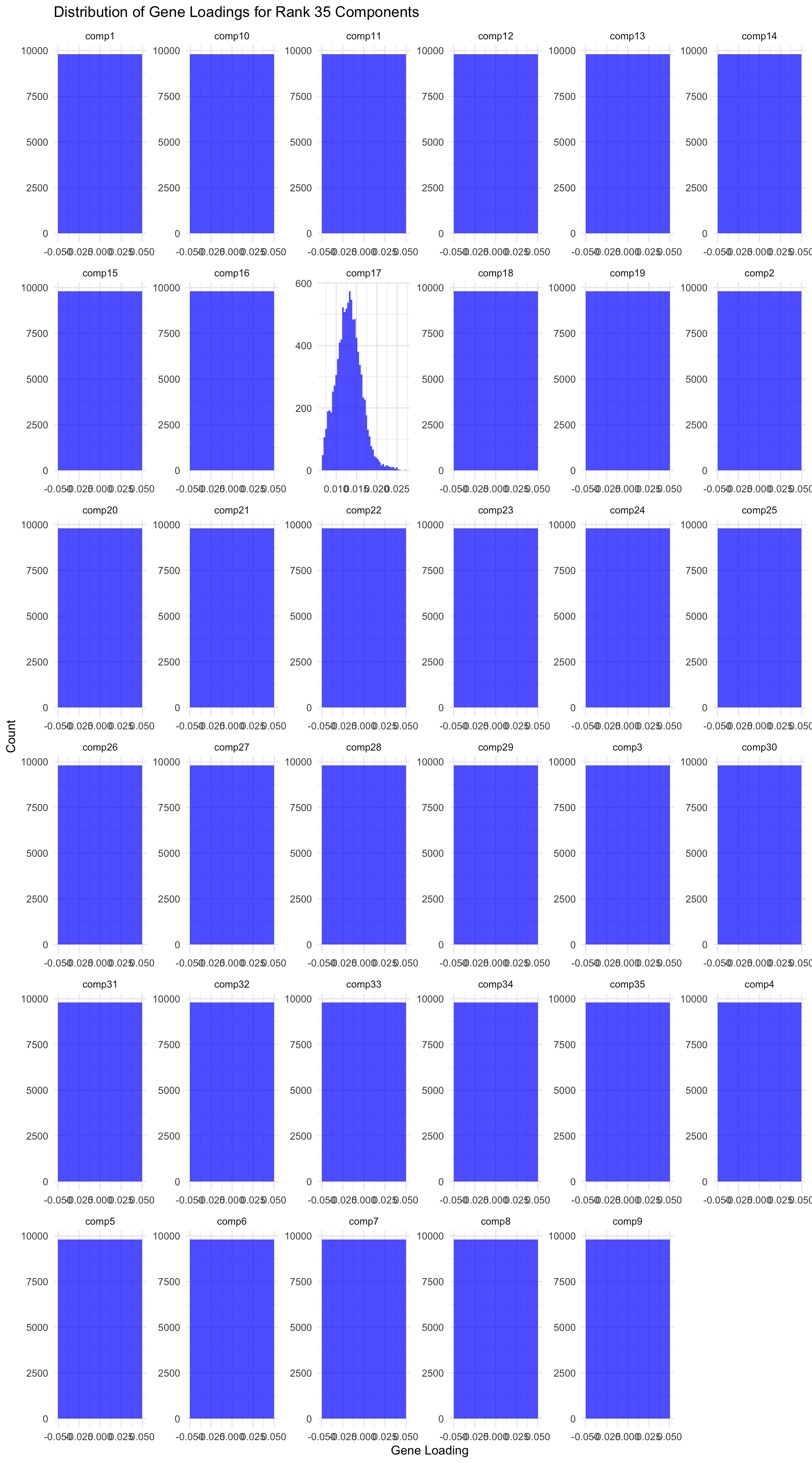
```{r, echo=TRUE, warning=FALSE, message=FALSE, fig.width=10, fig.height=18}
  # Load data
  gene_factors <- read_csv("https://gannet.fish.washington.edu/v1_web/owlshell/bu-github/timeseries_molecular/M-multi-species/output/40-rank35-optimization/lambda_gene_1000/barnacle_factors/gene_factors.csv")


#edit so columns names are shifted 1 to the left
  colnames(gene_factors) <- c("gene", paste0("comp", 1:(ncol(gene_factors)-1)))

#code to create histogram of gene_factors:

  library(ggplot2)
  library(tidyr)

  # Reshape data to long format
  gene_factors_long <- gene_factors %>%
    pivot_longer(cols = -1, names_to = "component", values_to = "loading")

  # Plot histogram
  ggplot(gene_factors_long, aes(x = loading)) +
    geom_histogram(bins = 50, fill = "blue", alpha = 0.7) +
    facet_wrap(~ component, scales = "free") +
    theme_minimal() +
    labs(title = "Distribution of Gene Loadings for Rank 35 Components",
         x = "Gene Loading",
         y = "Count")
```