---
title: "Barnacle"
description: "more lamda values"
categories: ["Transcriptomics"]
#citation:
date: 12-04-2025
image: http://gannet.fish.washington.edu/seashell/snaps/Monosnap_Image_2025-11-30_15-34-25.png # finding a good image
author:
- name: Steven Roberts
url:
orcid: 0000-0001-8302-1138
affiliation: Professor, UW - School of Aquatic and Fishery Sciences
affiliation-url: https://robertslab.info
#url: # self-defined
draft: false # setting this to `true` will prevent your post from appearing on your listing page until you're ready!
format:
html:
toc: true # ← enable TOC
toc-location: left # or: right, body
toc-depth: 3 # how many heading levels to show
code-fold: FALSE
code-tools: true
code-copy: true
highlight-style: github
code-overflow: wrap
#runtime: shiny
---
# More lamda testing
``` bash
LAMBDAS_GENE="1 2 4 6 8 10"
LAMBDA_SAMPLE=0.1
LAMBDA_TIME=0.05
RANK=35

mkdir -p ../output/41-rank35-optimization

OUTDIR_BASE=../output/41-rank35-optimization

for LG in $LAMBDAS_GENE; do
  OUTDIR=${OUTDIR_BASE}/lambda_gene_${LG}
  mkdir -p "$OUTDIR"

  uv run python ../scripts/14.1-barnacle/build_tensor_and_run.py \
    --input-file ../output/14-pca-orthologs/vst_counts_matrix.csv \
    --output-dir "$OUTDIR" \
    --rank $RANK \
    --lambda-gene $LG \
    --lambda-sample $LAMBDA_SAMPLE \
    --lambda-time $LAMBDA_TIME \
    --max-iter 1000 \
    --tol 1e-5 \
    --seed 92
done
```
```{r, echo=TRUE, warning=FALSE, message=FALSE}
library(tidyverse)

# ---------------------------------------------------------
# SETTINGS
# ---------------------------------------------------------

base_url <- "https://gannet.fish.washington.edu/v1_web/owlshell/bu-github/timeseries_molecular/M-multi-species/output/41-rank35-optimization"

lambda_vals <- c("1", "2", "4", "6", "8", "10")

# ---------------------------------------------------------
# FUNCTION: read gene_factors.csv AND FIX HEADER
# ---------------------------------------------------------
read_gene_factors <- function(lambda) {
  url <- sprintf("%s/lambda_gene_%s/barnacle_factors/gene_factors.csv",
                 base_url, lambda)

  message("Reading: ", url)
  df <- read_csv(url, show_col_types = FALSE)

  # Fix the shifted header here
  # First column should be "gene", others "comp1..compN"
  colnames(df) <- c("gene", paste0("comp", 1:(ncol(df)-1)))

  df$lambda_gene <- lambda
  df
}

# ---------------------------------------------------------
# READ ALL RUNS
# ---------------------------------------------------------
all_factors <- map_df(lambda_vals, read_gene_factors)

# ---------------------------------------------------------
# LONG FORMAT FOR ANALYSIS
# ---------------------------------------------------------
factor_long <- all_factors %>%
  pivot_longer(
    cols = starts_with("comp"),
    names_to = "component",
    values_to = "loading"
  )
```
```{r}
sparsity_tbl <- factor_long %>%
  group_by(lambda_gene) %>%
  summarize(
    n_values = n(),
    n_zero = sum(loading == 0 | abs(loading) < 1e-12),
    sparsity = n_zero / n_values
  )

sparsity_tbl
```
```{r}
gene_component_counts <- factor_long %>%
  filter(loading > 0) %>%
  group_by(lambda_gene, gene) %>%
  summarize(
    n_components = n_distinct(component),
    .groups = "drop"
  )
```
```{r}
multi_component_summary <- gene_component_counts %>%
  group_by(lambda_gene, n_components) %>%
  summarize(n_genes = n(), .groups = "drop")

multi_component_summary
```
```{r}
summary_tbl <- sparsity_tbl %>%
  left_join(
    gene_component_counts %>%
      group_by(lambda_gene) %>%
      summarize(
        mean_components = mean(n_components),
        frac_multi = mean(n_components > 1),
        .groups = "drop"
      ),
    by = "lambda_gene"
  )

summary_tbl
```
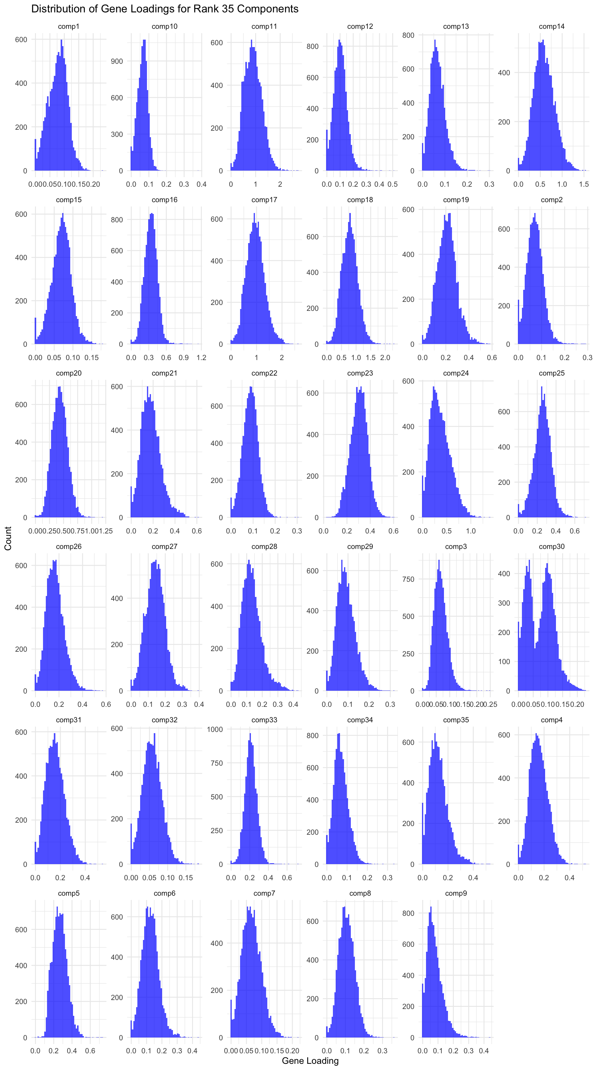
```{r, echo=TRUE, warning=FALSE, message=FALSE, fig.width=10, fig.height=18}
  # Load data
  gene_factors <- read_csv("https://gannet.fish.washington.edu/v1_web/owlshell/bu-github/timeseries_molecular/M-multi-species/output/41-rank35-optimization/lambda_gene_1/barnacle_factors/gene_factors.csv")


#edit so columns names are shifted 1 to the left
  colnames(gene_factors) <- c("gene", paste0("comp", 1:(ncol(gene_factors)-1)))

#code to create histogram of gene_factors:

  library(ggplot2)
  library(tidyr)

  # Reshape data to long format
  gene_factors_long <- gene_factors %>%
    pivot_longer(cols = -1, names_to = "component", values_to = "loading")

  # Plot histogram
  ggplot(gene_factors_long, aes(x = loading)) +
    geom_histogram(bins = 50, fill = "blue", alpha = 0.7) +
    facet_wrap(~ component, scales = "free") +
    theme_minimal() +
    labs(title = "Distribution of Gene Loadings for Rank 35 Components",
         x = "Gene Loading",
         y = "Count")
```
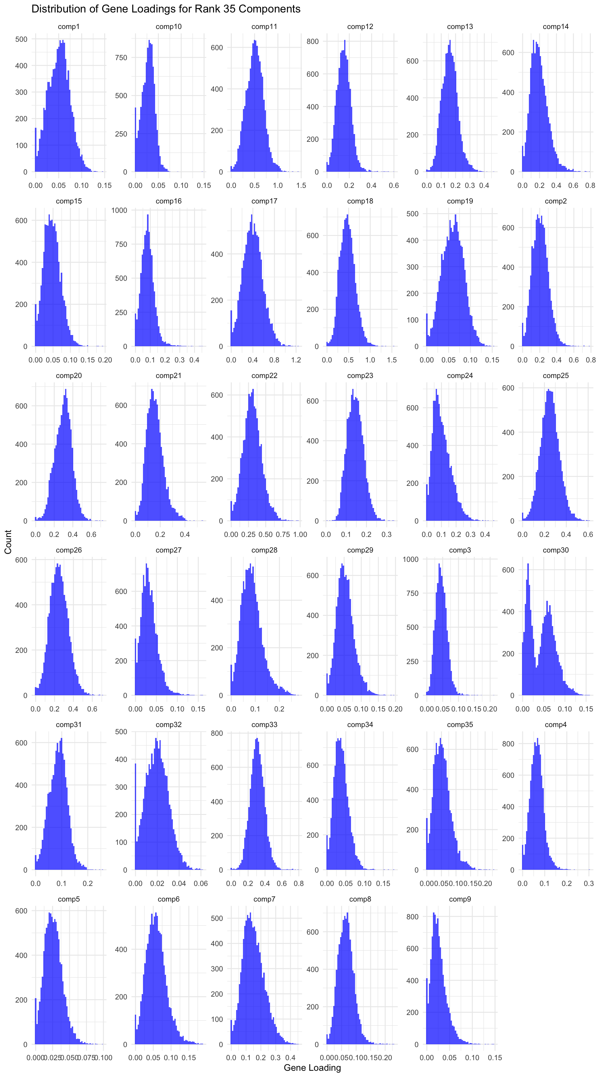
```{r, echo=TRUE, warning=FALSE, message=FALSE, fig.width=10, fig.height=18}
  # Load data
  gene_factors <- read_csv("https://gannet.fish.washington.edu/v1_web/owlshell/bu-github/timeseries_molecular/M-multi-species/output/41-rank35-optimization/lambda_gene_2/barnacle_factors/gene_factors.csv")


#edit so columns names are shifted 1 to the left
  colnames(gene_factors) <- c("gene", paste0("comp", 1:(ncol(gene_factors)-1)))

#code to create histogram of gene_factors:

  library(ggplot2)
  library(tidyr)

  # Reshape data to long format
  gene_factors_long <- gene_factors %>%
    pivot_longer(cols = -1, names_to = "component", values_to = "loading")

  # Plot histogram
  ggplot(gene_factors_long, aes(x = loading)) +
    geom_histogram(bins = 50, fill = "blue", alpha = 0.7) +
    facet_wrap(~ component, scales = "free") +
    theme_minimal() +
    labs(title = "Distribution of Gene Loadings for Rank 35 Components",
         x = "Gene Loading",
         y = "Count")
```
```{r, echo=TRUE, warning=FALSE, message=FALSE, fig.width=10, fig.height=18}
  # Load data
  gene_factors <- read_csv("https://gannet.fish.washington.edu/v1_web/owlshell/bu-github/timeseries_molecular/M-multi-species/output/41-rank35-optimization/lambda_gene_4/barnacle_factors/gene_factors.csv")


#edit so columns names are shifted 1 to the left
  colnames(gene_factors) <- c("gene", paste0("comp", 1:(ncol(gene_factors)-1)))

#code to create histogram of gene_factors:

  library(ggplot2)
  library(tidyr)

  # Reshape data to long format
  gene_factors_long <- gene_factors %>%
    pivot_longer(cols = -1, names_to = "component", values_to = "loading")

  # Plot histogram
  ggplot(gene_factors_long, aes(x = loading)) +
    geom_histogram(bins = 50, fill = "blue", alpha = 0.7) +
    facet_wrap(~ component, scales = "free") +
    theme_minimal() +
    labs(title = "Distribution of Gene Loadings for Rank 35 Components",
         x = "Gene Loading",
         y = "Count")
```
```{r, echo=TRUE, warning=FALSE, message=FALSE, fig.width=10, fig.height=18}
  # Load data
  gene_factors <- read_csv("https://gannet.fish.washington.edu/v1_web/owlshell/bu-github/timeseries_molecular/M-multi-species/output/41-rank35-optimization/lambda_gene_6/barnacle_factors/gene_factors.csv")


#edit so columns names are shifted 1 to the left
  colnames(gene_factors) <- c("gene", paste0("comp", 1:(ncol(gene_factors)-1)))

#code to create histogram of gene_factors:

  library(ggplot2)
  library(tidyr)

  # Reshape data to long format
  gene_factors_long <- gene_factors %>%
    pivot_longer(cols = -1, names_to = "component", values_to = "loading")

  # Plot histogram
  ggplot(gene_factors_long, aes(x = loading)) +
    geom_histogram(bins = 50, fill = "blue", alpha = 0.7) +
    facet_wrap(~ component, scales = "free") +
    theme_minimal() +
    labs(title = "Distribution of Gene Loadings for Rank 35 Components",
         x = "Gene Loading",
         y = "Count")
```
```{r, echo=TRUE, warning=FALSE, message=FALSE, fig.width=10, fig.height=18}
  # Load data
  gene_factors <- read_csv("https://gannet.fish.washington.edu/v1_web/owlshell/bu-github/timeseries_molecular/M-multi-species/output/41-rank35-optimization/lambda_gene_8/barnacle_factors/gene_factors.csv")


#edit so columns names are shifted 1 to the left
  colnames(gene_factors) <- c("gene", paste0("comp", 1:(ncol(gene_factors)-1)))

#code to create histogram of gene_factors:

  library(ggplot2)
  library(tidyr)

  # Reshape data to long format
  gene_factors_long <- gene_factors %>%
    pivot_longer(cols = -1, names_to = "component", values_to = "loading")

  # Plot histogram
  ggplot(gene_factors_long, aes(x = loading)) +
    geom_histogram(bins = 50, fill = "blue", alpha = 0.7) +
    facet_wrap(~ component, scales = "free") +
    theme_minimal() +
    labs(title = "Distribution of Gene Loadings for Rank 35 Components",
         x = "Gene Loading",
         y = "Count")
```
```{r, echo=TRUE, warning=FALSE, message=FALSE, fig.width=10, fig.height=18}
  # Load data
  gene_factors <- read_csv("https://gannet.fish.washington.edu/v1_web/owlshell/bu-github/timeseries_molecular/M-multi-species/output/41-rank35-optimization/lambda_gene_10/barnacle_factors/gene_factors.csv")


#edit so columns names are shifted 1 to the left
  colnames(gene_factors) <- c("gene", paste0("comp", 1:(ncol(gene_factors)-1)))

#code to create histogram of gene_factors:

  library(ggplot2)
  library(tidyr)

  # Reshape data to long format
  gene_factors_long <- gene_factors %>%
    pivot_longer(cols = -1, names_to = "component", values_to = "loading")

  # Plot histogram
  ggplot(gene_factors_long, aes(x = loading)) +
    geom_histogram(bins = 50, fill = "blue", alpha = 0.7) +
    facet_wrap(~ component, scales = "free") +
    theme_minimal() +
    labs(title = "Distribution of Gene Loadings for Rank 35 Components",
         x = "Gene Loading",
         y = "Count")
```