
Two lake trout ecotypes, two hifiasm assemblies, and one question: do the lean and siscowet genomes agree on gene order, and how does each line up against the reference? This is the gene-anchored synteny pass (Track B of the ecotype genome-comparison plan). The trick that makes it cheap is that orthology is already solved — Liftoff gave every lifted gene the reference gene-XXX ID, so a gene shared between two genomes carries the same base ID. That means MCScanX anchor pairs can be synthesized straight from ID identity, with no OrthoFinder / DIAMOND step.
Full outputs (too large for GitHub) live on gannet.
Step 1 — Purge haplotigs
The raw hifiasm assemblies were size-inflated relative to the ~2.5 Gb expected genome, a classic sign of retained haplotigs that would show up as spurious duplications in any synteny map. So each assembly went through the standard purge_dups HiFi pipeline (map reads back for depth → cutoffs → self-align → purge → extract primary set) before anything else.
| Ecotype | Raw | Purged |
|---|---|---|
| lean | 3.73 Gb / 33,035 contigs | 2.58 Gb / 12,700 contigs |
| siscowet | 4.0 Gb / 24,184 contigs | 2.84 Gb / 8,159 contigs |
That knocked lean down to essentially the expected genome size and roughly halved the contig count for both.
Step 2 — Re-lift the annotation
Gene coordinates have to match the sequences being compared, so I re-ran Liftoff (same flags: -polish -copies -sc 0.95 -u) against the purged FASTAs and pulled a genes-only BED per ecotype.
- lean: 55,437 lifted genes (4,636 unmapped)
- siscowet: 59,968 lifted genes (3,069 unmapped)
Step 3–4 — Synthetic anchors + MCScanX
Instead of running an aligner to find homologs, I built the MCScanX .blast files by joining the per-genome gene maps on their base ID (stripping the _N copy suffix Liftoff adds, so gene-family expansions still form multiple pairs). Genome codes (rf, ln, si) prefix every chromosome tag and gene UID so MCScanX can tell intra- from inter-genome blocks, and the . in accessions like NC_052307.1 gets stripped since MCScanX chokes on it.
Three comparisons, all anchored to the same 42-chromosome reference:
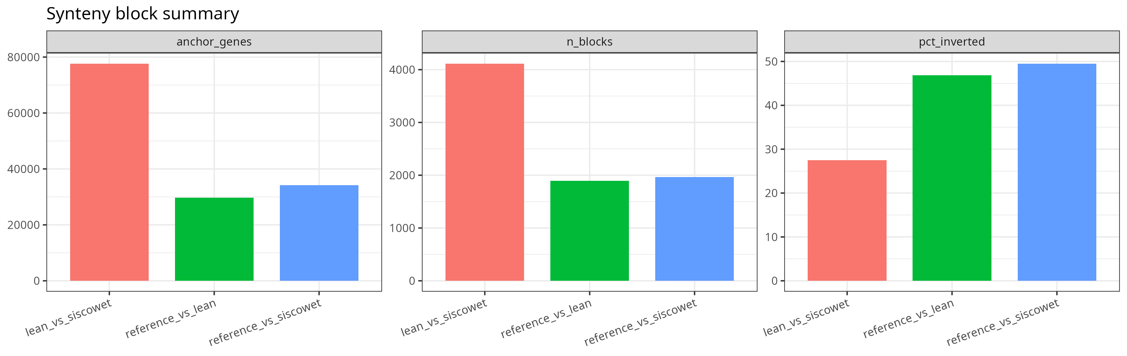
| Comparison | Collinear blocks | Anchor genes | Inverted blocks |
|---|---|---|---|
| reference vs lean | 1,897 | 29,695 | 889 |
| reference vs siscowet | 1,966 | 34,231 | 973 |
| lean vs siscowet | 4,113 | 77,628 | 1,130 |
The cross-ecotype comparison (lean vs siscowet) is the richest — nearly 78k anchor genes across 4,113 blocks — which is what you’d hope for between two assemblies of the same species. The reference comparisons are more fragmented, as expected given the reference is chromosome-scale while the ecotype assemblies are still contigs.
Step 5–6 — Summarize and plot
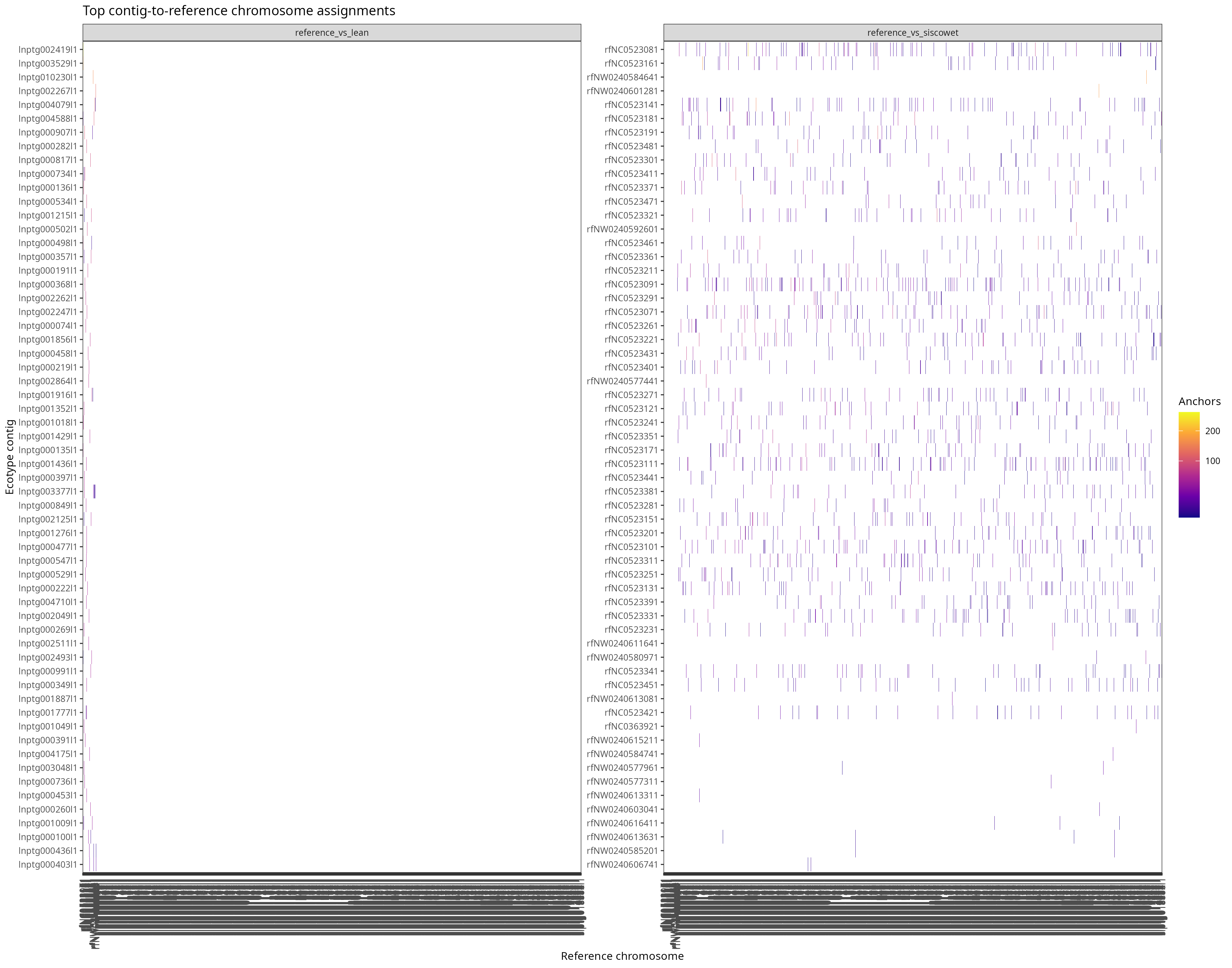
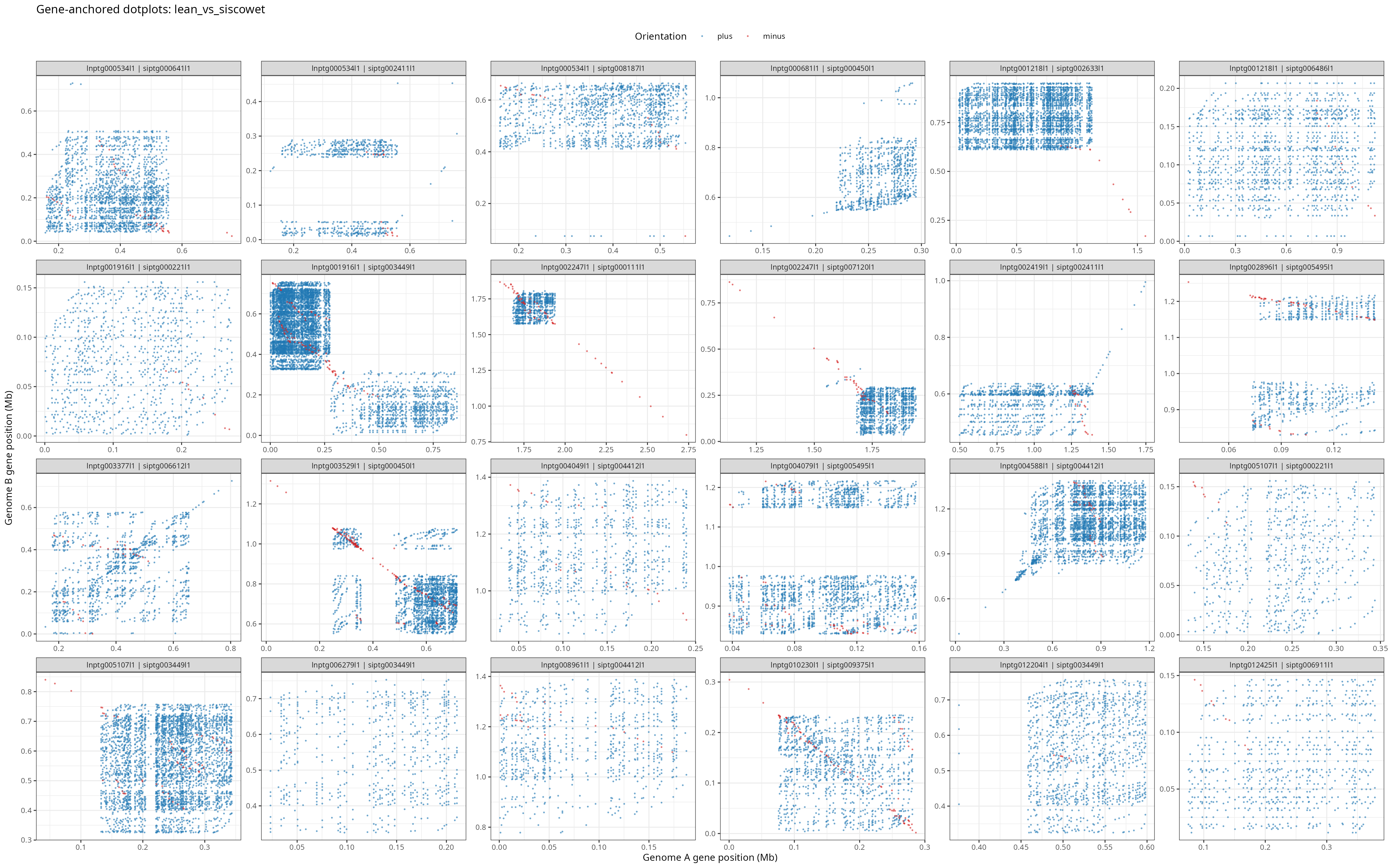
Each .collinearity was parsed into a tidy block table (synteny_blocks.tsv) and a contig-to-reference-chromosome assignment (contig_to_chromosome.tsv), then three figure types were rendered to plots/:
- Comparison summary bars — blocks, anchor genes, % inverted per comparison.
- Contig-to-chromosome heatmaps — which ecotype contig maps to which reference chromosome.
- Gene-level dotplots — anchor positions per chromosome pair, colored by orientation.
Deliverables
Written to output/21.1-gene-anchored-synteny/:
{eco}.purged.fa— haplotig-purged primary assemblies{eco}.purged.liftoff.genes.bed— re-lifted genes on the purged assemblies{ref_lean,ref_sisco,lean_sisco}.collinearity— MCScanX collinear blockssynteny_blocks.tsv— tidy block table (chromosomes, anchor counts, orientation)contig_to_chromosome.tsv— ecotype contig → reference chromosome assignment
These feed the structural-variant and overlay steps next — whole-genome alignment (Track A), plus PAV and DMR overlay.
In plain English
A few terms from the table above:
Anchor genes — genes we could confidently match up as “the same gene” in both genomes being compared. These are the shared landmarks. The more anchors, the more the two genomes have in common. Between the two ecotypes we found ~78,000 of them.
Collinear blocks — runs of anchor genes that appear in the same order in both genomes. A block is a stretch where the layout is conserved, like a passage of text that reads identically in both books. Thousands of blocks means large parts of the genome are laid out the same way in both fish.
Inverted blocks — blocks where the genes are the same and still in order, but the whole segment is flipped end-for-end (like a paragraph printed backwards). This happens when a chunk of DNA gets reversed during evolution. Tracking these tells us where the two genomes have been rearranged rather than simply copied.
One housekeeping step worth explaining: the raw genome drafts were nearly twice as big as they should be. That’s because the sequencing captured both copies of each chromosome (one from each parent) and sometimes listed them as if they were separate pieces — inflating the total. Purging removes those redundant copies so we’re comparing one clean version of each genome, not a genome accidentally doubled up.