
The question
Lean and siscowet lake trout are two ecotypes of the same species that look and behave differently — siscowet are deep-water, fat-rich fish; lean are shallower-water and leaner. Earlier work in this project (21.1) matched up genes between the two ecotypes and the reference genome, one gene at a time. That tells us which genes correspond to each other, but not how the genome itself has been rearranged — whether whole chunks of DNA have flipped around, moved to a different chromosome, or been duplicated. That’s what this step, described in full in 23.1-genome-sv-map.Rmd, is for.
What’s a “structural variant”?
Most genetic differences people think of are tiny — a single letter (base) swapped for another (a SNP). Structural variants (SVs) are the bigger, chunkier kind of difference:
- Inversion — a segment of DNA is flipped end-to-end.
- Translocation — a segment moved to a different location or chromosome.
- Duplication — a segment copied, so it appears more than once.
- Indel — a stretch of DNA inserted or deleted.
- Diverged / highly-diverged regions — stretches that aligned but accumulated a lot of small differences.
Any of these can disrupt, duplicate, or relocate genes — which makes them good candidates for explaining trait differences between ecotypes that a single-gene comparison would miss.
How we found them
- Anchor each ecotype’s genome onto the 42 reference chromosomes using RagTag, so lean, siscowet, and the reference all share the same chromosome-numbering scheme.
- Align each pair of genomes whole-genome, base-by-base, with minimap2.
- Call variants on those alignments with SyRI, a tool built specifically to sort genome differences into syntenic (matching) blocks versus the SV categories above.
- Summarize and plot the results.
Three comparisons were run: lean-vs-reference, siscowet-vs-reference, and lean-vs-siscowet directly. (At the time of this writing, siscowet-vs-reference is still processing — the numbers and plots below cover lean-vs-reference and the direct lean-vs-siscowet comparison.)
What we found
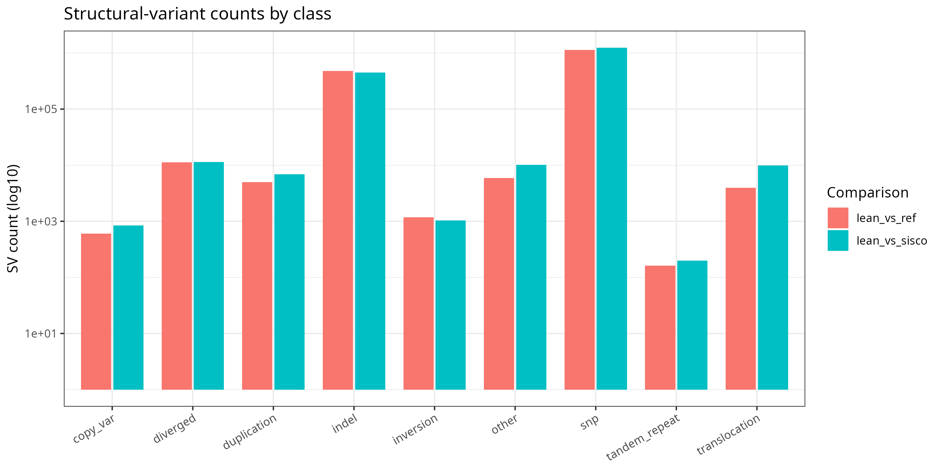
How much of the genome is rearranged?
Both comparisons turn up thousands of inversions, duplications, and translocations, plus hundreds of thousands of small indels — but lean-vs-siscowet (comparing the two ecotypes directly) consistently shows more rearrangements than either ecotype does against the reference. That’s expected: the reference is more closely related to one lineage, so ecotype-vs-ecotype differences stack the changes from both branches together.
How much DNA is actually involved?
Counting events is one thing; some SVs are a few bases, others span megabases. This plot shows the total amount of reference genome sequence (in Mb) covered by each SV class:
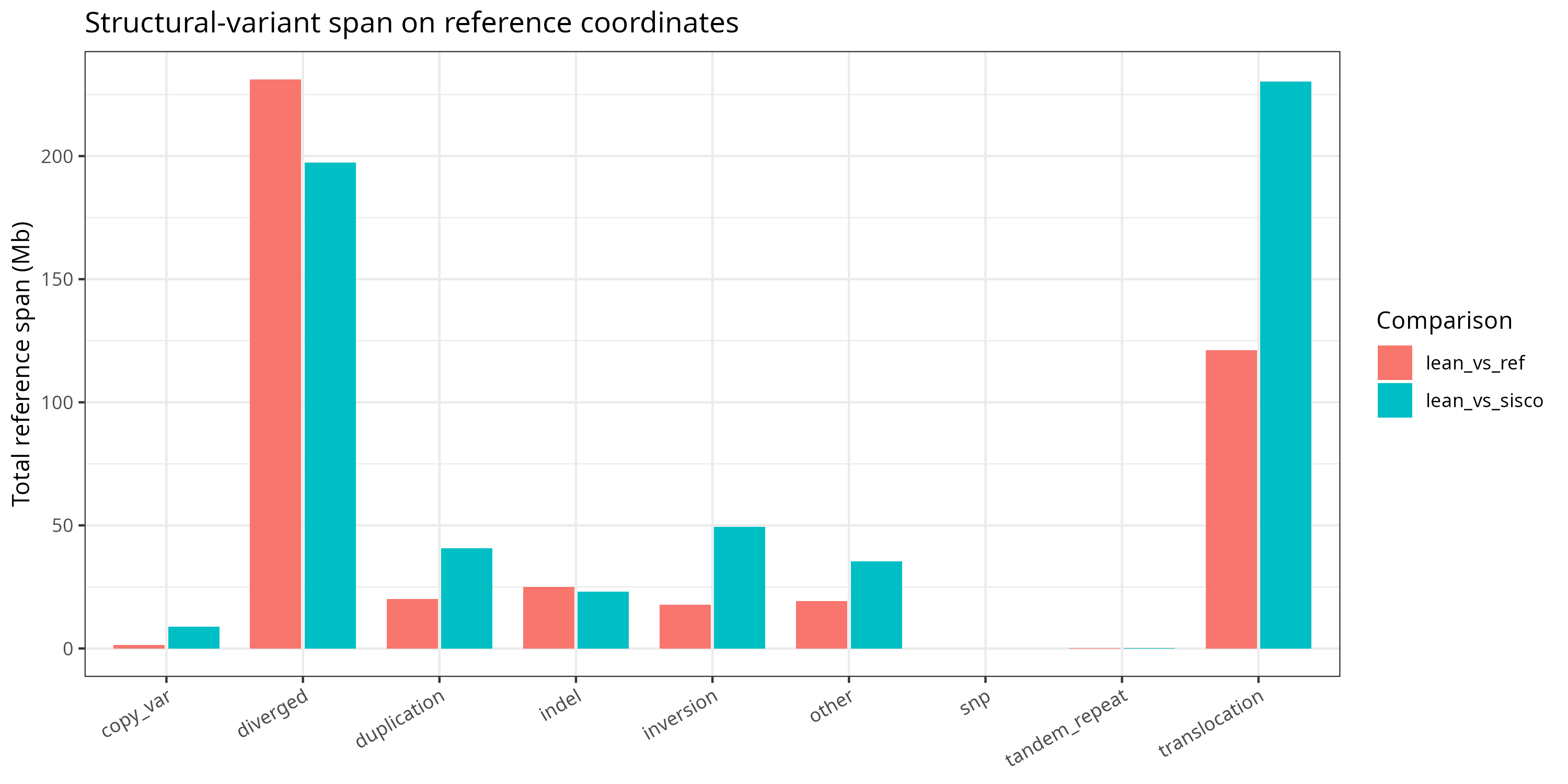
Translocations and highly-diverged regions dominate by footprint — in the lean-vs-siscowet comparison, translocated segments alone total roughly 230 Mb, and diverged regions another ~197 Mb, out of a ~2.5–2.8 Gb genome. Inversions cover tens of megabases in both comparisons. So while indels are the most numerous SV type, translocations and inversions are the ones that move around the most sequence.
What it looks like across the genome
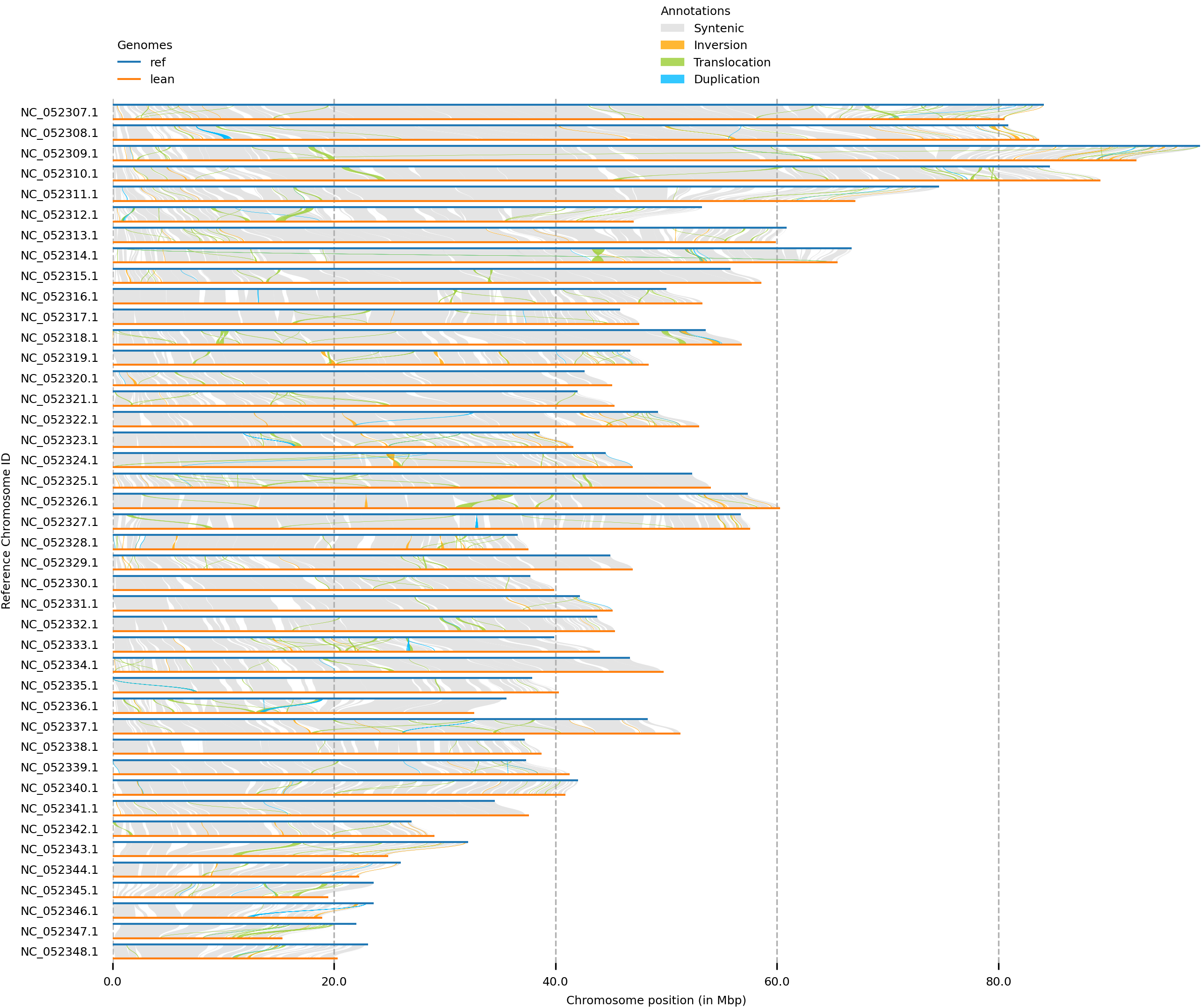
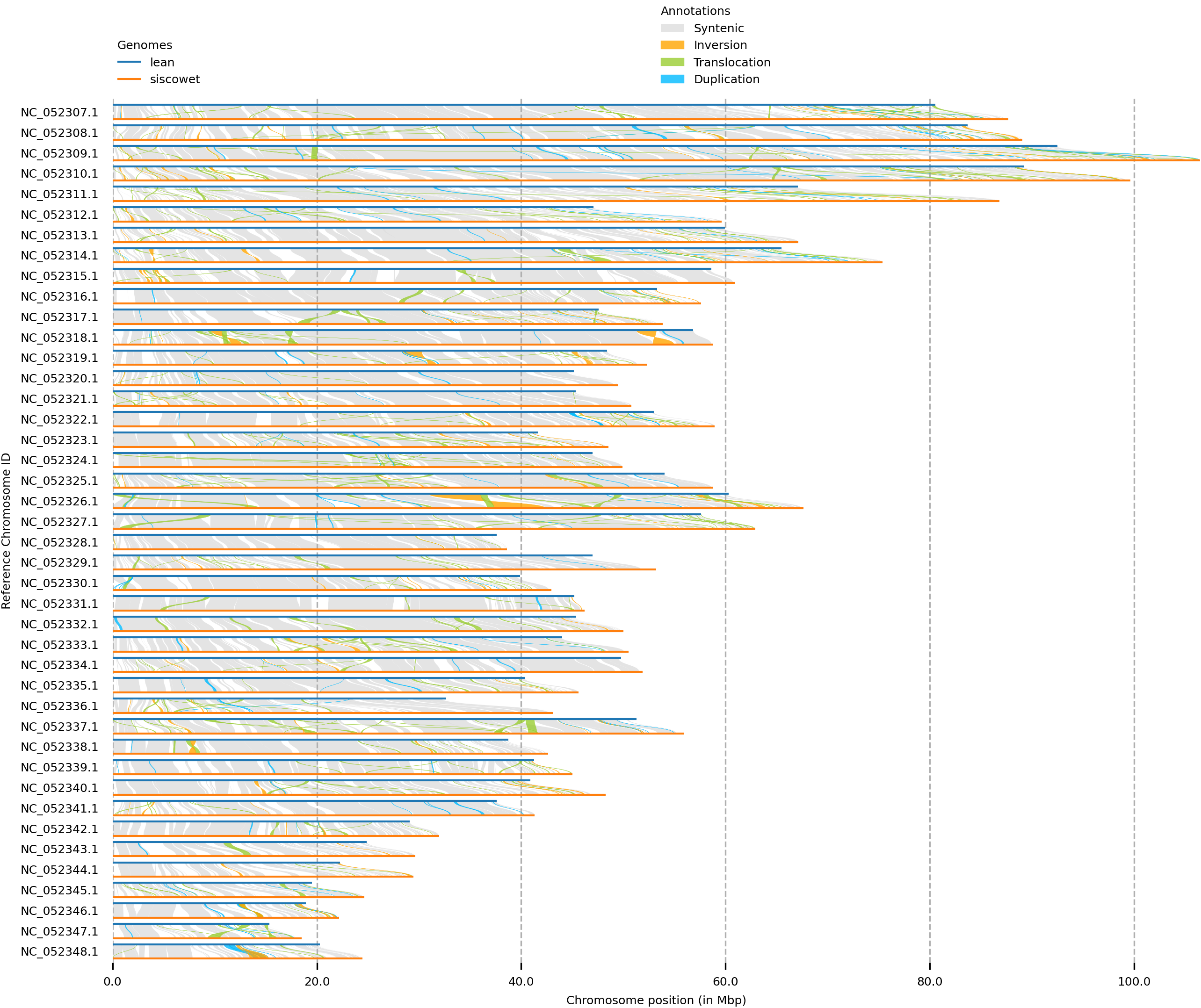
The plots below (from plotsr) lay both genomes side by side, chromosome by chromosome, and draw a ribbon between every matching segment — colored by whether it’s syntenic (gray), inverted, translocated, or duplicated. This is the most intuitive view: you can see directly which chromosomes have large flipped or relocated blocks.
Lean vs. reference:
Lean vs. siscowet:
Checking our work against an independent method
A separate, earlier analysis (15-diff-pav.py) had already flagged regions present in one ecotype but absent in another (presence/absence variation, or PAV) just by comparing coverage against the reference — a much simpler method than SyRI’s full alignment. Cross-validating the two (23.2-sv-pav-crossvalidate.py) asks: of the regions PAV flagged, how many does SyRI independently confirm as a real structural event?
| Ecotype | PAV-flagged regions | Confirmed by SyRI | Fraction confirmed |
|---|---|---|---|
| lean insertions | 770,891 | 141,159 | 18.3% |
| lean deletions | 225,337 | 45,948 | 20.4% |
Roughly a fifth of the PAV calls line up with a SyRI-confirmed structural variant — mostly highly-diverged regions, duplications, and translocations. That’s a meaningful overlap given the two methods work completely differently (read-depth/coverage vs. full alignment), and it gives us a high-confidence subset of SVs that two independent approaches agree on.
Why this matters
This is the first sequence-level, whole-genome map of how the lean and siscowet genomes differ structurally — not just gene-by-gene, but at the level of entire rearranged segments. It completes the piece of the ecotype comparison that gene-anchored synteny alone couldn’t answer, and gives us a shortlist of large, high-confidence structural differences to check against the gene annotations for candidates that might relate to the depth and body-fat differences between the two ecotypes.
What’s next
- Finish the siscowet-vs-reference comparison and fold it into the summary and plots above.
- Feed the confirmed SVs into the genome browsers alongside the gene-anchored synteny tracks (22-synteny-browser-integration), so a rearrangement and the genes inside it can be viewed together.
- Look for genes that fall inside the largest, high-confidence inversions/translocations as candidates worth a closer look.
All large intermediate files (alignments, full SyRI output, etc.) are too big for GitHub and are hosted instead at gannet.fish.washington.edu/gitrepos/project-lake-trout/analyses/23-genome-sv/.