
1 Run HiSat on RNA-seq
Will end up with 5 sorted bam files.
1.1 Grab Trimmed RNA-seq Reads
ls ../data/fastq/ RNA-ACR-140-S1-TP2_R1_001.fastp-trim.20230519.fastq.gz
RNA-ACR-140-S1-TP2_R2_001.fastp-trim.20230519.fastq.gz
RNA-ACR-145-S1-TP2_R1_001.fastp-trim.20230519.fastq.gz
RNA-ACR-145-S1-TP2_R2_001.fastp-trim.20230519.fastq.gz
RNA-ACR-150-S1-TP2_R1_001.fastp-trim.20230519.fastq.gz
RNA-ACR-150-S1-TP2_R2_001.fastp-trim.20230519.fastq.gz
RNA-ACR-173-S1-TP2_R1_001.fastp-trim.20230519.fastq.gz
RNA-ACR-173-S1-TP2_R2_001.fastp-trim.20230519.fastq.gz
RNA-ACR-178-S1-TP2_R1_001.fastp-trim.20230519.fastq.gz
RNA-ACR-178-S1-TP2_R2_001.fastp-trim.20230519.fastq.gz1.2 Genome
ls ../data/GCF_013753865.1_Amil_v2.1_genomic.fna../data/GCF_013753865.1_Amil_v2.1_genomic.fnahead ../data/Amil/ncbi_dataset/data/GCF_013753865.1/genomic.gtf
wc -l ../data/Amil/ncbi_dataset/data/GCF_013753865.1/genomic.gtf
grep -v '^#' ../data/Amil/ncbi_dataset/data/GCF_013753865.1/genomic.gtf | cut -f3 | sort | uniq
grep -c "transcript" ../data/Amil/ncbi_dataset/data/GCF_013753865.1/genomic.gtf
grep -c "gene" ../data/Amil/ncbi_dataset/data/GCF_013753865.1/genomic.gtf#gtf-version 2.2
#!genome-build Amil_v2.1
#!genome-build-accession NCBI_Assembly:GCF_013753865.1
#!annotation-source NCBI Acropora millepora Annotation Release 101
NC_058066.1 Gnomon gene 1962 23221 . - . gene_id "LOC114963522"; transcript_id ""; db_xref "GeneID:114963522"; gbkey "Gene"; gene "LOC114963522"; gene_biotype "lncRNA";
NC_058066.1 Gnomon transcript 1962 23221 . - . gene_id "LOC114963522"; transcript_id "XR_003825913.2"; db_xref "GeneID:114963522"; gbkey "ncRNA"; gene "LOC114963522"; model_evidence "Supporting evidence includes similarity to: 100% coverage of the annotated genomic feature by RNAseq alignments, including 2 samples with support for all annotated introns"; product "uncharacterized LOC114963522"; transcript_biotype "lnc_RNA";
NC_058066.1 Gnomon exon 23085 23221 . - . gene_id "LOC114963522"; transcript_id "XR_003825913.2"; db_xref "GeneID:114963522"; gene "LOC114963522"; model_evidence "Supporting evidence includes similarity to: 100% coverage of the annotated genomic feature by RNAseq alignments, including 2 samples with support for all annotated introns"; product "uncharacterized LOC114963522"; transcript_biotype "lnc_RNA"; exon_number "1";
NC_058066.1 Gnomon exon 21001 21093 . - . gene_id "LOC114963522"; transcript_id "XR_003825913.2"; db_xref "GeneID:114963522"; gene "LOC114963522"; model_evidence "Supporting evidence includes similarity to: 100% coverage of the annotated genomic feature by RNAseq alignments, including 2 samples with support for all annotated introns"; product "uncharacterized LOC114963522"; transcript_biotype "lnc_RNA"; exon_number "2";
NC_058066.1 Gnomon exon 18711 18775 . - . gene_id "LOC114963522"; transcript_id "XR_003825913.2"; db_xref "GeneID:114963522"; gene "LOC114963522"; model_evidence "Supporting evidence includes similarity to: 100% coverage of the annotated genomic feature by RNAseq alignments, including 2 samples with support for all annotated introns"; product "uncharacterized LOC114963522"; transcript_biotype "lnc_RNA"; exon_number "3";
NC_058066.1 Gnomon exon 1962 2119 . - . gene_id "LOC114963522"; transcript_id "XR_003825913.2"; db_xref "GeneID:114963522"; gene "LOC114963522"; model_evidence "Supporting evidence includes similarity to: 100% coverage of the annotated genomic feature by RNAseq alignments, including 2 samples with support for all annotated introns"; product "uncharacterized LOC114963522"; transcript_biotype "lnc_RNA"; exon_number "4";
874259 ../data/Amil/ncbi_dataset/data/GCF_013753865.1/genomic.gtf
CDS
exon
gene
start_codon
stop_codon
transcript
874254
874254head ../data/Amil/ncbi_dataset/data/GCF_013753865.1/genomic.gff
wc -l ../data/Amil/ncbi_dataset/data/GCF_013753865.1/genomic.gff
grep -v '^#' ../data/Amil/ncbi_dataset/data/GCF_013753865.1/genomic.gff | cut -f3 | sort | uniq
grep -c "transcript" ../data/Amil/ncbi_dataset/data/GCF_013753865.1/genomic.gff
grep -c "gene" ../data/Amil/ncbi_dataset/data/GCF_013753865.1/genomic.gff##gff-version 3
#!gff-spec-version 1.21
#!processor NCBI annotwriter
#!genome-build Amil_v2.1
#!genome-build-accession NCBI_Assembly:GCF_013753865.1
#!annotation-source NCBI Acropora millepora Annotation Release 101
##sequence-region NC_058066.1 1 39361238
##species https://www.ncbi.nlm.nih.gov/Taxonomy/Browser/wwwtax.cgi?id=45264
NC_058066.1 RefSeq region 1 39361238 . + . ID=NC_058066.1:1..39361238;Dbxref=taxon:45264;Name=1;chromosome=1;collection-date=2017;country=Indonesia;gbkey=Src;genome=chromosome;isolate=JS-1;isolation-source=Whole tissue;mol_type=genomic DNA;tissue-type=Adult tissue
NC_058066.1 Gnomon gene 1962 23221 . - . ID=gene-LOC114963522;Dbxref=GeneID:114963522;Name=LOC114963522;gbkey=Gene;gene=LOC114963522;gene_biotype=lncRNA
828216 ../data/Amil/ncbi_dataset/data/GCF_013753865.1/genomic.gff
cDNA_match
CDS
exon
gene
guide_RNA
lnc_RNA
mRNA
pseudogene
region
rRNA
snoRNA
snRNA
transcript
tRNA
431975
8032601.3 HiSat
/home/shared/hisat2-2.2.1/hisat2_extract_exons.py \
../data/Amil/ncbi_dataset/data/GCF_013753865.1/genomic.gtf \
> ../output/15-Apul-hisat/m_exon.tab
head ../output/15-Apul-hisat/m_exon.tab
wc -l ../output/15-Apul-hisat/m_exon.tabNC_058066.1 1961 2118 -
NC_058066.1 15360 15663 +
NC_058066.1 18710 18774 -
NC_058066.1 21000 21092 -
NC_058066.1 22158 22442 +
NC_058066.1 23084 23220 -
NC_058066.1 24770 25066 +
NC_058066.1 26652 26912 +
NC_058066.1 27071 27358 +
NC_058066.1 27658 27951 +
228010 ../output/15-Apul-hisat/m_exon.tab
/home/shared/hisat2-2.2.1/hisat2_extract_splice_sites.py \
../data/Amil/ncbi_dataset/data/GCF_013753865.1/genomic.gtf \
> ../output/15-Apul-hisat/m_splice_sites.tab
head ../output/15-Apul-hisat/m_splice_sites.tabNC_058066.1 2118 18710 -
NC_058066.1 15663 22158 +
NC_058066.1 18774 21000 -
NC_058066.1 21092 23084 -
NC_058066.1 22442 24770 +
NC_058066.1 25066 26652 +
NC_058066.1 26912 27071 +
NC_058066.1 27358 27658 +
NC_058066.1 27951 28247 +
NC_058066.1 28534 29196 +/home/shared/hisat2-2.2.1/hisat2-build \
../data/GCF_013753865.1_Amil_v2.1_genomic.fna \
../output/15-Apul-hisat/GCF_013753865.1_Amil_v2.1.index \
--exon ../output/15-Apul-hisat/m_exon.tab \
--ss ../output/15-Apul-hisat/m_splice_sites.tab \
-p 40 \
../data/Amil/ncbi_dataset/data/GCF_013753865.1/genomic.gtf \
2> ../output/15-Apul-hisat/hisat2-build_stats.txttail ../output/15-Apul-hisat/hisat2-build_stats.txt sideSz: 128
sideGbwtSz: 104
sideGbwtLen: 208
numSides: 2299750
numLines: 2299750
gbwtTotLen: 294368000
gbwtTotSz: 294368000
reverse: 0
linearFM: No
Total time for call to driver() for forward index: 00:07:581.3.1 Performance tuning
If your computer has multiple processors/cores, use -p The -p option causes HISAT2 to launch a specified number of parallel search threads. Each thread runs on a different processor/core and all threads find alignments in parallel, increasing alignment throughput by approximately a multiple of the number of threads (though in practice, speedup is somewhat worse than linear).
find ../data/fastq/*R2_001.fastp-trim.20230519.fastq.gz \
| xargs basename -s -S1-TP2_R2_001.fastp-trim.20230519.fastq.gz | xargs -I{} \
/home/shared/hisat2-2.2.1/hisat2 \
-x ../output/15-Apul-hisat/GCF_013753865.1_Amil_v2.1.index \
--dta \
-p 20 \
-1 ../data/fastq/{}-S1-TP2_R1_001.fastp-trim.20230519.fastq.gz \
-2 ../data/fastq/{}-S1-TP2_R2_001.fastp-trim.20230519.fastq.gz \
-S ../output/15-Apul-hisat/{}.sam \
2> ../output/15-Apul-hisat/hisat.out
cat ../output/15-Apul-hisat/hisat.out47710408 reads; of these:
47710408 (100.00%) were paired; of these:
27825914 (58.32%) aligned concordantly 0 times
18559152 (38.90%) aligned concordantly exactly 1 time
1325342 (2.78%) aligned concordantly >1 times
----
27825914 pairs aligned concordantly 0 times; of these:
1201636 (4.32%) aligned discordantly 1 time
----
26624278 pairs aligned 0 times concordantly or discordantly; of these:
53248556 mates make up the pairs; of these:
42533390 (79.88%) aligned 0 times
9692346 (18.20%) aligned exactly 1 time
1022820 (1.92%) aligned >1 times
55.43% overall alignment rate
42864294 reads; of these:
42864294 (100.00%) were paired; of these:
24356414 (56.82%) aligned concordantly 0 times
17135863 (39.98%) aligned concordantly exactly 1 time
1372017 (3.20%) aligned concordantly >1 times
----
24356414 pairs aligned concordantly 0 times; of these:
1142678 (4.69%) aligned discordantly 1 time
----
23213736 pairs aligned 0 times concordantly or discordantly; of these:
46427472 mates make up the pairs; of these:
36609836 (78.85%) aligned 0 times
8675847 (18.69%) aligned exactly 1 time
1141789 (2.46%) aligned >1 times
57.30% overall alignment rate
43712298 reads; of these:
43712298 (100.00%) were paired; of these:
30967520 (70.84%) aligned concordantly 0 times
11666917 (26.69%) aligned concordantly exactly 1 time
1077861 (2.47%) aligned concordantly >1 times
----
30967520 pairs aligned concordantly 0 times; of these:
791338 (2.56%) aligned discordantly 1 time
----
30176182 pairs aligned 0 times concordantly or discordantly; of these:
60352364 mates make up the pairs; of these:
52153613 (86.42%) aligned 0 times
7011301 (11.62%) aligned exactly 1 time
1187450 (1.97%) aligned >1 times
40.34% overall alignment rate
47501524 reads; of these:
47501524 (100.00%) were paired; of these:
28603496 (60.22%) aligned concordantly 0 times
17627744 (37.11%) aligned concordantly exactly 1 time
1270284 (2.67%) aligned concordantly >1 times
----
28603496 pairs aligned concordantly 0 times; of these:
1201709 (4.20%) aligned discordantly 1 time
----
27401787 pairs aligned 0 times concordantly or discordantly; of these:
54803574 mates make up the pairs; of these:
44045470 (80.37%) aligned 0 times
9614980 (17.54%) aligned exactly 1 time
1143124 (2.09%) aligned >1 times
53.64% overall alignment rate
42677752 reads; of these:
42677752 (100.00%) were paired; of these:
26422177 (61.91%) aligned concordantly 0 times
15005422 (35.16%) aligned concordantly exactly 1 time
1250153 (2.93%) aligned concordantly >1 times
----
26422177 pairs aligned concordantly 0 times; of these:
1009838 (3.82%) aligned discordantly 1 time
----
25412339 pairs aligned 0 times concordantly or discordantly; of these:
50824678 mates make up the pairs; of these:
39698309 (78.11%) aligned 0 times
9739502 (19.16%) aligned exactly 1 time
1386867 (2.73%) aligned >1 times
53.49% overall alignment rate1.4 convert to bam
for samfile in ../output/15-Apul-hisat/*.sam; do
  bamfile="${samfile%.sam}.bam"
  sorted_bamfile="${samfile%.sam}.sorted.bam"
  /home/shared/samtools-1.12/samtools view -bS -@ 20 "$samfile" > "$bamfile"
  /home/shared/samtools-1.12/samtools sort -@ 20 "$bamfile" -o "$sorted_bamfile"
  /home/shared/samtools-1.12/samtools index -@ 20 "$sorted_bamfile"
done
1.5 Looking at Bams
\[igv\]
1.5.0.1 Differential expression analysis
Together with HISAT and Ballgown, StringTie can be used for estimating differential expression across multiple RNA-Seq samples and generating plots and differential expression tables as described in our protocol paper.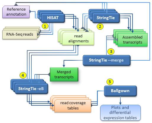
Our recommended workflow includes the following steps:
for each RNA-Seq sample, map the reads to the genome with HISAT2 using the –dta option. It is highly recommended to use the reference annotation information when mapping the reads, which can be either embedded in the genome index (built with the –ss and –exon options, see HISAT2 manual), or provided separately at run time (using the –known-splicesite-infile option of HISAT2). The SAM output of each HISAT2 run must be sorted and converted to BAM using samtools as explained above.
for each RNA-Seq sample, run StringTie to assemble the read alignments obtained in the previous step; it is recommended to run StringTie with the -G option if the reference annotation is available.
run StringTie with –merge in order to generate a non-redundant set of transcripts observed in any of the RNA-Seq samples assembled previously. The stringtie –merge mode takes as input a list of all the assembled transcripts files (in GTF format) previously obtained for each sample, as well as a reference annotation file (-G option) if available.
for each RNA-Seq sample, run StringTie using the -B/-b and -e options in order to estimate transcript abundances and generate read coverage tables for Ballgown. The -e option is not required but recommended for this run in order to produce more accurate abundance estimations of the input transcripts. Each StringTie run in this step will take as input the sorted read alignments (BAM file) obtained in step 1 for the corresponding sample and the -G option with the merged transcripts (GTF file) generated by stringtie –merge in step 3. Please note that this is the only case where the -G option is not used with a reference annotation, but with the global, merged set of transcripts as observed across all samples. (This step is the equivalent of the Tablemaker step described in the original Ballgown pipeline.)
Ballgown can now be used to load the coverage tables generated in the previous step and perform various statistical analyses for differential expression, generate plots etc.
1.5.1 An alternate, faster differential expression analysis workflow
can be pursued if there is no interest in novel isoforms (i.e. assembled transcripts present in the samples but missing from the reference annotation), or if only a well known set of transcripts of interest are targeted by the analysis. This simplified protocol has only 3 steps (depicted below) as it bypasses the individual assembly of each RNA-Seq sample and the “transcript merge” step.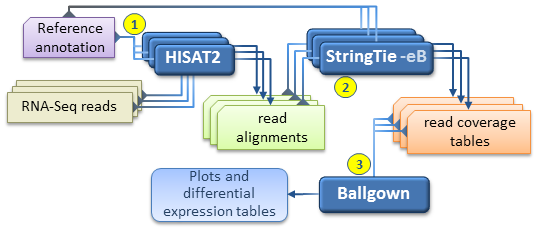 This simplified workflow attempts to directly estimate and analyze the expression of a known set of transcripts as given in the reference annotation file.
The R package IsoformSwitchAnalyzeR can be used to assign gene names to transcripts assembled by StringTie, which can be particularly helpful in cases where StringTie could not perform this assignment unambigiously.
The importIsoformExpression() + importRdata() function of the package can be used to import the expression and annotation data into R. During this import the package will attempt to clean up and recover isoform annotations where possible. From the resulting switchAnalyzeRlist object, IsoformSwitchAnalyzeR can detect isoform switches along with predicted functional consequences. The extractGeneExpression() function can be used to get a gene expression (read count) matrix for analysis with other tools.
More information and code examples can be found here.
2 StringTie
StringTie uses the sorted BAM files to assemble transcripts for each sample, outputting them as GTF files. And then merges all individual GTF assemblies into a single merged GTF file. This step extracts transcript information and merges GTFs from all samples–an important step in creating a canonical list of across all samples included in the pipeline.
| -b <path> | Just like -B this option enables the output of *.ctab files for Ballgown, but these files will be created in the provided directory <path> instead of the directory specified by the -o option. Note: adding the -e option is recommended with the -B/-b options, unless novel transcripts are still wanted in the StringTie GTF output. |
-e |
this option directs StringTie to operate in expression estimation mode; this limits the processing of read alignments to estimating the coverage of the transcripts given with the -G option (hence this option requires -G). |
| -G <ref_ann.gff> | Use a reference annotation file (in GTF or GFF3 format) to guide the assembly process. The output will include expressed reference transcripts as well as any novel transcripts that are assembled. This option is required by options -B, -b, -e, -C (see below). |
find ../output/15-Apul-hisat/*sorted.bam \
| xargs basename -s .sorted.bam | xargs -I{} \
/home/shared/stringtie-2.2.1.Linux_x86_64/stringtie \
-p 20 \
-eB \
-G ../data/Amil/ncbi_dataset/data/GCF_013753865.1/genomic.gff \
-o ../output/15-Apul-hisat/{}.gtf \
../output/15-Apul-hisat/{}.sorted.bam
wc -l ../output/15-Apul-hisat/RNA*.gtf
ls ../output/15-Apul-hisat/RNA*.gtf
#head ../output/15-Apul-hisat/RNA*.gtf 445208 ../output/15-Apul-hisat/RNA-ACR-140.gtf
445208 ../output/15-Apul-hisat/RNA-ACR-145.gtf
445208 ../output/15-Apul-hisat/RNA-ACR-150.gtf
445208 ../output/15-Apul-hisat/RNA-ACR-173.gtf
445208 ../output/15-Apul-hisat/RNA-ACR-178.gtf
2226040 total
../output/15-Apul-hisat/RNA-ACR-140.gtf
../output/15-Apul-hisat/RNA-ACR-145.gtf
../output/15-Apul-hisat/RNA-ACR-150.gtf
../output/15-Apul-hisat/RNA-ACR-173.gtf
../output/15-Apul-hisat/RNA-ACR-178.gtfThe R package IsoformSwitchAnalyzeR can be used to assign gene names to transcripts assembled by StringTie, which can be particularly helpful in cases where StringTie could not perform this assignment unambigiously.
The importIsoformExpression() + importRdata() function of the package can be used to import the expression and annotation data into R. During this import the package will attempt to clean up and recover isoform annotations where possible. From the resulting switchAnalyzeRlist object, IsoformSwitchAnalyzeR can detect isoform switches along with predicted functional consequences. The extractGeneExpression() function can be used to get a gene expression (read count) matrix for analysis with other tools.
More information and code examples can be found here.
2.0.1 Using StringTie with DESeq2 and edgeR
DESeq2 and edgeR are two popular Bioconductor packages for analyzing differential expression, which take as input a matrix of read counts mapped to particular genomic features (e.g., genes). We provide a Python script (prepDE.py, or the Python 3 version:prepDE.py3 ) that can be used to extract this read count information directly from the files generated by StringTie (run with the -e parameter).
prepDE.py derives hypothetical read counts for each transcript from the coverage values estimated by StringTie for each transcript, by using this simple formula: reads_per_transcript = coverage * transcript_len / read_len
There are two ways to provide input to the prepDE.py script:
one option is to provide a path to a directory containing all sample sub-directories, with the same structure as the ballgowndirectory in the StringTie protocol paper in preparation for Ballgown. By default (no -i option), the script is going to look in the current directory for all sub-directories having .gtf files in them, as in this example:
    ./sample1/sample1.gtf
    ./sample2/sample2.gtf
    ./sample3/sample3.gtf
Alternatively, one can provide a text file listing sample IDs and their respective paths (sample_lst.txt).
Usage: prepDE.py options
generates two CSV files containing the count matrices for genes and transcripts, using the coverage values found in the output of stringtie -e
Options:
-h, –help show this help message and exit
-i INPUT, a folder containing all sample sub-directories, or a –input=INPUT, text file with sample ID and path to its GTF file on –in=INPUT each line default:.
-g G where to output the gene count matrix default:genecountmatrix.csv
-t T where to output the transcript count matrix default:transcriptcountmatrix.csv
-l LENGTH, the average read length default:75–length=LENGTH
-p PATTERN, a regular expression that selects the sample –pattern=PATTERN subdirectories
-c, –cluster whether to cluster genes that overlap with different gene IDs, ignoring ones with geneID pattern (see below)
-s STRING, if a different prefix is used for geneIDs assigned by –string=STRING StringTie default:MSTRG
-k KEY, –key=KEY if clustering, what prefix to use for geneIDs assigned by this script default:prepG
–legend=LEGEND if clustering, where to output the legend file mapping transcripts to assigned geneIDs default:legend.csv——————– ——————————————————
These count matrices (CSV files) can then be imported into R for use by DESeq2 and edgeR (using the DESeqDataSetFromMatrix and DGEList functions, respectively).
2.0.1.0.1 Protocol: Using StringTie with DESeq2
Given a list of GTFs, which were re-estimated upon merging, users can follow the below protocol to use DESeq2 for differential expression analysis. To generate GTFs from raw reads follow the StringTie protocol paper (up to the Ballgown step).
As described above, prepDE.py either accepts a .txt (sample_lst.txt) file listing the sample IDs and the GTFs’ paths or by default expects a ballgown directory produced by StringTie run with the -B option. The following steps leads us through generating count matrices for genes and transcripts, importing this data into DESeq2, and conducting some basic analysis.
Generate count matrices using prepDE.py
Assuming default ballgown directory structure produced by StringTie
$ python prepDE.pyList of GTFs sample IDs and paths (sample_lst.txt)
$ python prepDE.py -i sample_lst.txt
Install R and DESeq2. Upon installing R, install DESeq2 on R:
> source("https://bioconductor.org/biocLite.R")> biocLite("DESeq2")Import DESeq2 library in R
> library("DESeq2")Load gene(/transcript) count matrix and labels
> countData <- as.matrix(read.csv("gene_count_matrix.csv", row.names="gene_id"))> colData <- read.csv(PHENO_DATA, sep="\t", row.names=1)
Note: The PHENO_DATA file contains information on each sample, e.g., sex or population. The exact way to import this depends on the format of the file.Check all sample IDs in colData are also in CountData and match their orders
> all(rownames(colData) %in% colnames(countData))1TRUE
> countData <- countData[, rownames(colData)]> all(rownames(colData) == colnames(countData))1TRUECreate a DESeqDataSet from count matrix and labels
> dds <- DESeqDataSetFromMatrix(countData = countData, colData = colData, design = ~ CHOOSE_FEATURE)Run the default analysis for DESeq2 and generate results table
> dds <- DESeq(dds)> res <- results(dds)Sort by adjusted p-value and display
> (resOrdered <- res[order(res$padj), ])
python /home/shared/stringtie-2.2.1.Linux_x86_64/prepDE.py python /home/shared/stringtie-2.2.1.Linux_x86_64/prepDE.py \
-i ../data/list01.txt \
-g ../output/15-Apul-hisat/gene_count_matrix.csv \
-t ../output/15-Apul-hisat/transcript_count_matrix.csv3 DESeq
library(DESeq2)# Load gene(/transcript) count matrix and labels
countData <- as.matrix(read.csv("../output/15-Apul-hisat/gene_count_matrix.csv", row.names="gene_id"))
colData <- read.csv("../data/conditions.txt", sep="\t", row.names=1)
# Note: The PHENO_DATA file contains information on each sample, e.g., sex or population.
# The exact way to import this depends on the format of the file.
# Check all sample IDs in colData are also in CountData and match their orders
all(rownames(colData) %in% colnames(countData)) # This should return TRUE[1] TRUEcountData <- countData[, rownames(colData)]
all(rownames(colData) == colnames(countData)) # This should also return TRUE[1] TRUE# Create a DESeqDataSet from count matrix and labels
dds <- DESeqDataSetFromMatrix(countData = countData,
colData = colData, design = ~ Condition)
# Run the default analysis for DESeq2 and generate results table
dds <- DESeq(dds)
deseq2.res <- results(dds)
# Sort by adjusted p-value and display
resOrdered <- deseq2.res[order(deseq2.res$padj), ]vsd <- vst(dds, blind = FALSE)
plotPCA(vsd, intgroup = "Condition")
tmp <- deseq2.res
# The main plot
plot(tmp$baseMean, tmp$log2FoldChange, pch=20, cex=0.45, ylim=c(-3, 3), log="x", col="darkgray",
     main="DEG Dessication  (pval <= 0.05)",
     xlab="mean of normalized counts",
     ylab="Log2 Fold Change")
# Getting the significant points and plotting them again so they're a different color
tmp.sig <- deseq2.res[!is.na(deseq2.res$padj) & deseq2.res$padj <= 0.05, ]
points(tmp.sig$baseMean, tmp.sig$log2FoldChange, pch=20, cex=0.45, col="red")
# 2 FC lines
abline(h=c(-1,1), col="blue")