Bioinformatics Class Projects
Another quarter is complete for our Bioinformatics class , and once again we learned a bit.
This was the general plan…
| Week | Description | Reading | Quiz |
|---|---|---|---|
| zero | Biology, Course Framework, Getting set-up | Preface xiii-xxv; How to Learn Bioinformatics 1-18 | Questions |
| one | Bash, version control, Project Set-up | Setting Up and Managing a Bioinformatics Project 21-35; Remedial Unix Shell 37-54 | Questions |
| two | Jupyter, Annotation | Retrieving Bioinformatics Data 109-124, Unix Data tools 125-168 | Questions |
| three | Projects | Working with Sequence Data 339-354 | Questions |
| four | RNA-seq | Git for Scientists 67-83 | Questions |
| five | lncRNA miRNA | Working with Remote Machines 57-66 | Questions |
| six | DNA methylation | Gavery Slides | Questions |
| seven | Genome Browser | Working with Alignment Data 355-383, Working with Range Data 329-338 | Questions |
| eight | Holiday | :turkey: :turkey: 🌽 🍰 💻 | |
| nine | SNP | Bioinformatics Shell Scripting, Writing Pipelines 395-423 | Questions |
And everyone had a course repo
- hputnam
- yaaminiv
- mmiddleton
- aspanjer
- jldimond
- mfisher5
- nclowell
- laurahspencer
- Ellior2
- MeganEDuffy
- sr320
That resulted into a “Final Product” by the end.
Here are the highlights of everyone’s efforts.
@MeganEDuffy was quite committed, examining the metaproteomic profile in the Eastern Tropical Pacific Oxygen Minimum Zone.
Duffy, Megan (2016): Metaproteomic profile of an OMZ, version 1. figshare. https://dx.doi.org/10.6084/m9.figshare.4428059.v1 Retrieved: 15 19, Dec 19, 2016 (GMT)
The three underlying goals:
-
Complete both database searching based and de novo sequencing protein identifications for a series of seven depths (55 m to 2500 m) from the Eastern Tropical North Pacific (ETNP) oxygen minimum zone. Compare the quality of identifications from each method and with depth.
-
Use identified proteins and peptides to get a sense of microbial diversity compared with oxygen concentration.
-
Compare the ability of de novo peptide sequencing and database searching to identify E. coli peptide standards
One of many of the findings:
@laurahspencer annotated the draft Geoduck genome.
![]()
laurahspencer. (2016). laurahspencer/546-Bioinformatics: Final Project: Geoduck Genome Annotation of >70k bp Scaffolds [Data set]. Zenodo. http://doi.org/10.5281/zenodo.203660
This release includes final project files associated with the annotation of large scaffolds of the Panopea generosa (geoduck) genome. Release files include detailed workflows documented in Jupyter Notebooks, intermediate files, and availability of all source data. Products include:
- Subset of the genome with only >70k bp scaffolds
- Blast alignment of transcriptome to genome scaffolds
- Merged file with transcriptome annotations indexed on genome scaffolds; includes Uniprot data, bp sequences, and start & end sites for both transcriptome & genome
- Candidate Transposable elements, via RepeatMasker.
- Candidate Methylation sites (CpGs) - via Galaxy’s EMBOSS fuzznuc tool.
- Candidate miRNA sites - via miRBase;
- RNASeq reads from male & female gonad tissue aligned to genome scaffolds - via bowtie2 & samtools
- SNP sites called via samtools & bcftools
- IGV session with tracks from all the above data, linked to URLs on GitHub and lab web server.
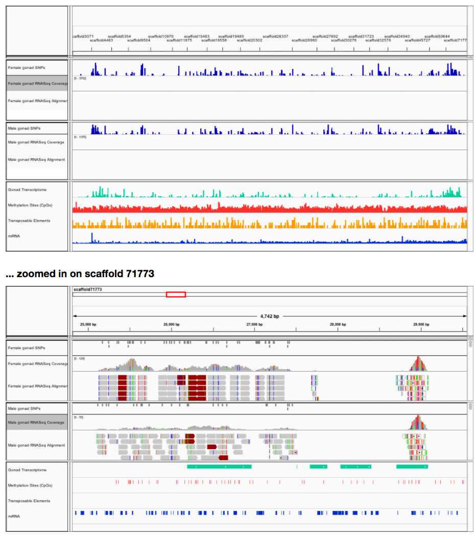
If you want to play with the data yourself in IGV, all you have to do is
File > Load from url
https://raw.githubusercontent.com/laurahspencer/546-Bioinformatics/bdb305054204c872ffb3c06f6404b17c3b29517c/2016-10_Geo-Ann-Project/results/09-Pg_70k_tracks.xml

@mmiddleton described a Oncorhynchus mykiss sperm methylome.
![]()
mmiddleton. (2016). mmiddleton/mmiddleton-fish546: O.mykiss sperm methylome [Data set]. Zenodo. http://doi.org/10.5281/zenodo.203574
DNA methylation was assessed with Bismark on both the CoGe platform and locally.

Parameters used to extract methylation information:
Bismark Extractor Version: v0.16.3
Bismark result file: single-end (SAM format)
Output specified: comprehensive


Processed 2779453 lines in total
Total number of methylation call strings processed: 2779453

Final Cytosine Methylation Report
=================================
Total number of C's analysed:	87198646

Total methylated C's in CpG context:	11732428
Total methylated C's in CHG context:	103618
Total methylated C's in CHH context:	227242

Total C to T conversions in CpG context:	2401136
Total C to T conversions in CHG context:	19981462
Total C to T conversions in CHH context:	52752760

C methylated in CpG context:	83.0%
C methylated in CHG context:	0.5%
C methylated in CHH context:	0.4%
@aspanger looked at Coho salmon differential expression analysis across a land use gradient in freshwater streams.
He pushed 18 commits to master and 18 commits to all branches. On master, 1,818 files have changed and there have been 1,420,664 additions and 924,335 deletions.
Coho Salmon (Oncorhynchus kisutch) are heavily dependent on small stream habitat for rearing, spending over a year in these habitats before out migrating. These fresh water habitats are susceptible to anthropogenic impact from structural changes to habitat, temperature effects from increased runoff and reduced canopy cover, flow changes, and an increased presence of toxicants both from point and non-point sources. As such, Coho health can serve of an indication of anthropogenic influence in these habitats and are of great interest due to their cultural and commercial importance.
This project uses sequencing data from coho collected at four streams spanning an urban impact gradient. The objectives are:
- Construct a de novo transcriptome for a non-sequenced species.
- Use the annotated Rainbow Trout and Atlantic Salmon genomes to annotate the resulting transcriptome.
- Conduct differential expression analysis between habitat conditions with the intent of identifying biomarkers indicative of toxicant exposure, immune deficiencies, and temperature stress.
- Use Gene Ontology analysis to explore the biological function of observed gene expression differences and to help explain the transcriptome in the context of other sequencing work that’s been completed on coho.
There was lots of data that informed
and at the end of the quarter, there were several circles.
more at GitHub - aspanjer/RNAseq_Coho
and this is what the repo structure looks like
Analysis: the results of each analytical step to complete the above objectives (e.g. FastQC results, trimmed sequencing files, etc)
BlastDB: the unique species specific blast databases used for annotating the transcriptome
Data_raw: the 48 raw PE sequencing files for each of the 24 sampled individual fish. (available on request)
Jupyter_notebook: contains the notebooks for my class project. Focuses on the de novo assembly of a coho transcriptome and subsequent differential expression analysis and annotation:
DataQC and Trinity Prep Differential Expression Annotation Gene Ontology
Scripts: Scripts used for analysis that aren’t download directly to my computer through Anaconda (these will be documented in my notebook).
Screenshots: pictures for analysis documentation
mfisher tackled some RAD-seq on Pacific cod around the Korean peninsula. Specifically she wanted to clarify population structure of Pacific cod spawning aggregates in South Korean waters.
![]()
mfisher5. (2016). mfisher5/mf-fish546-PCod: Pacific Cod RADseq Project, FISH546 [Data set]. Zenodo. http://doi.org/10.5281/zenodo.203351
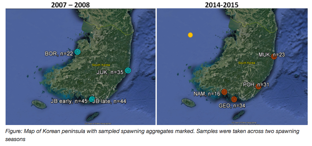
Lots of fun stuff to see including
With a great readme to take you where you want to go
from said page
Class Objectives:
(1) Become familiar with the stacks pipeline using Lane 1 sequence data
Jupyter notebook <br
(2) Optimize parameters for stacks pipeline
(a) Research previous papers / labmate work on parameters for c and ustacks, and come up with a list of parameter values to test.
    (b) Determine quantitative measures that will be used for comparing different batches of c/ustacks parameters

    (c) Run through stacks with the Lane 1 data  *Jupyter notebook [p1](https://github.com/mfisher5/mf-fish546-PCod/blob/master/notebooks/testing%20stacks/Testing%20stacks%20Parameters%20I%20.ipynb)*, *[p2](https://github.com/mfisher5/mf-fish546-PCod/blob/master/notebooks/testing%20stacks/Testing%20stacks%20Parameters%20II.ipynb)*

    (d) Analyze output to decide which parameters to use going forward   *[Evernote](https://www.evernote.com/shard/s650/sh/138af148-ea28-416e-b79d-2550b2829d50/3dd0a2619d17e859)*
<br
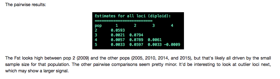
(3) Get a preliminary analysis of population structure between 7 populations in the Lanes 1 and 2 data. Here is a helpful workflow diagram of population structure analysis, including links to examples of what stacks output looks like.
   (a) Run through the full `stacks` pipeline with Lanes 1 and 2 data  *[Jupyter notebook](https://github.com/mfisher5/mf-fish546-PCod/blob/master/notebooks/Lanes%201%20and%202%20combined%20pipeline.ipynb)*

   (b) Obtain measures of population structure (paired and overall Fst), and conduct Discriminant Analysis of Principle Components (DAPC)  *[Jupyter notebook](https://github.com/mfisher5/mf-fish546-PCod/blob/master/notebooks/Lanes%201%20and%202%20combined%2C%20Analyses%20%2B%20Results.ipynb)*  <br
(4) Compare sequencing output from 300ng and degraded DNA protocols to determine if these protocols will be used on the rest of the samples.
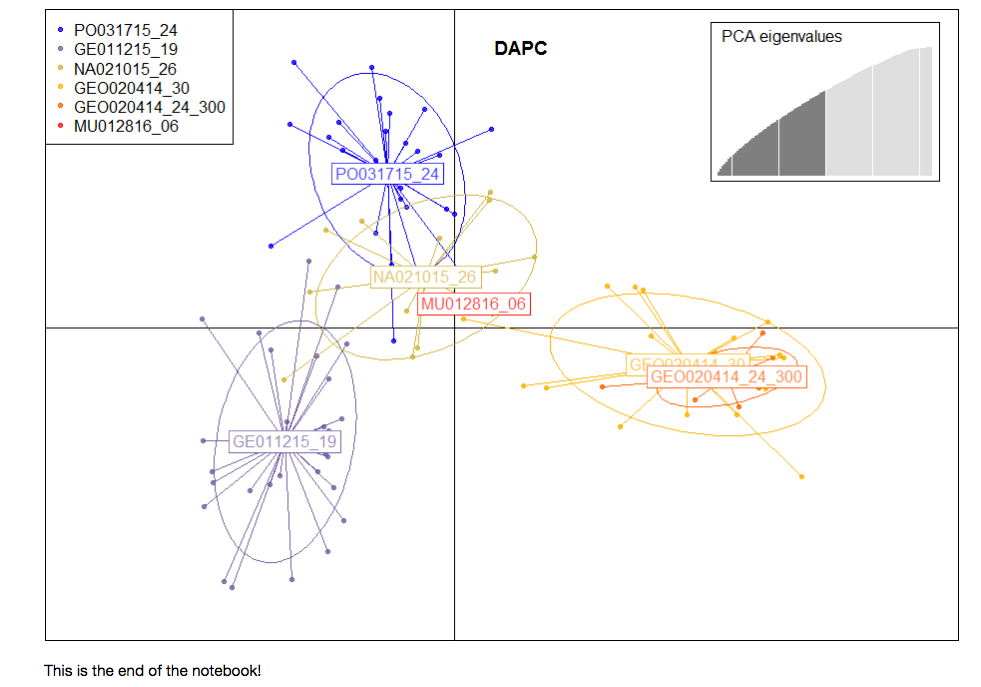
@nclowell set out to measure adaptive difference within and between cohorts of Pacific cod in the Salish Sea using RADseq data.
![]()
Natalie Lowell. (2016). FISH 546 Final Project [Data set]. Zenodo. http://doi.org/10.5281/zenodo.203291

There is some great stuff in here. i.e.
And be sure to check out the Readme.md with a nice reflection of the quarter
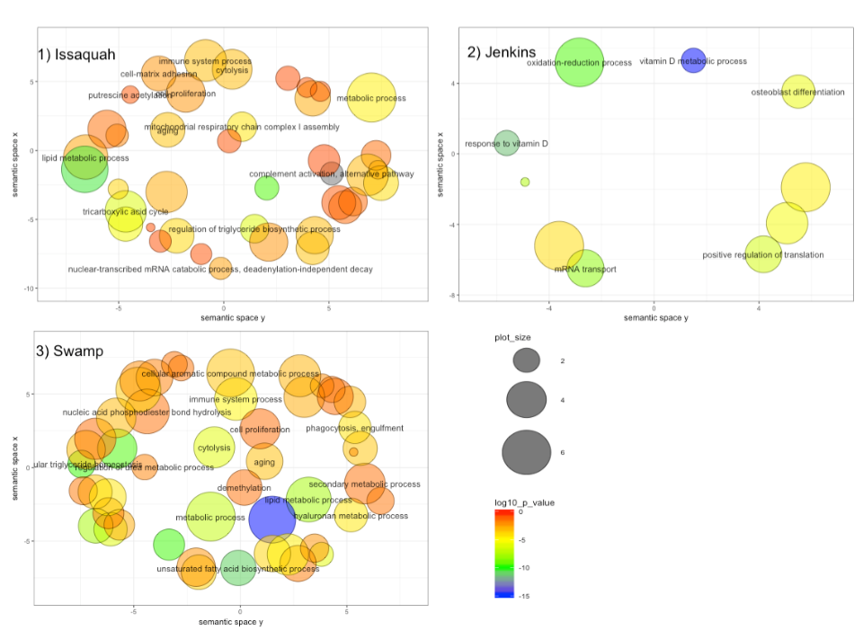
@Ellior2 annotated the Pacific oyster Crassostrea gigas proteome
![]()
Rhonda Elliott, mmiddleton, & laurahspencer. (2016). Ellior2/Fish-546-Bioinformatics: Characterization of Pacific oyster proteome- Final Draft [Data set]. Zenodo. http://doi.org/10.5281/zenodo.202894
Goals (via Readme.md )
My goals for this course:
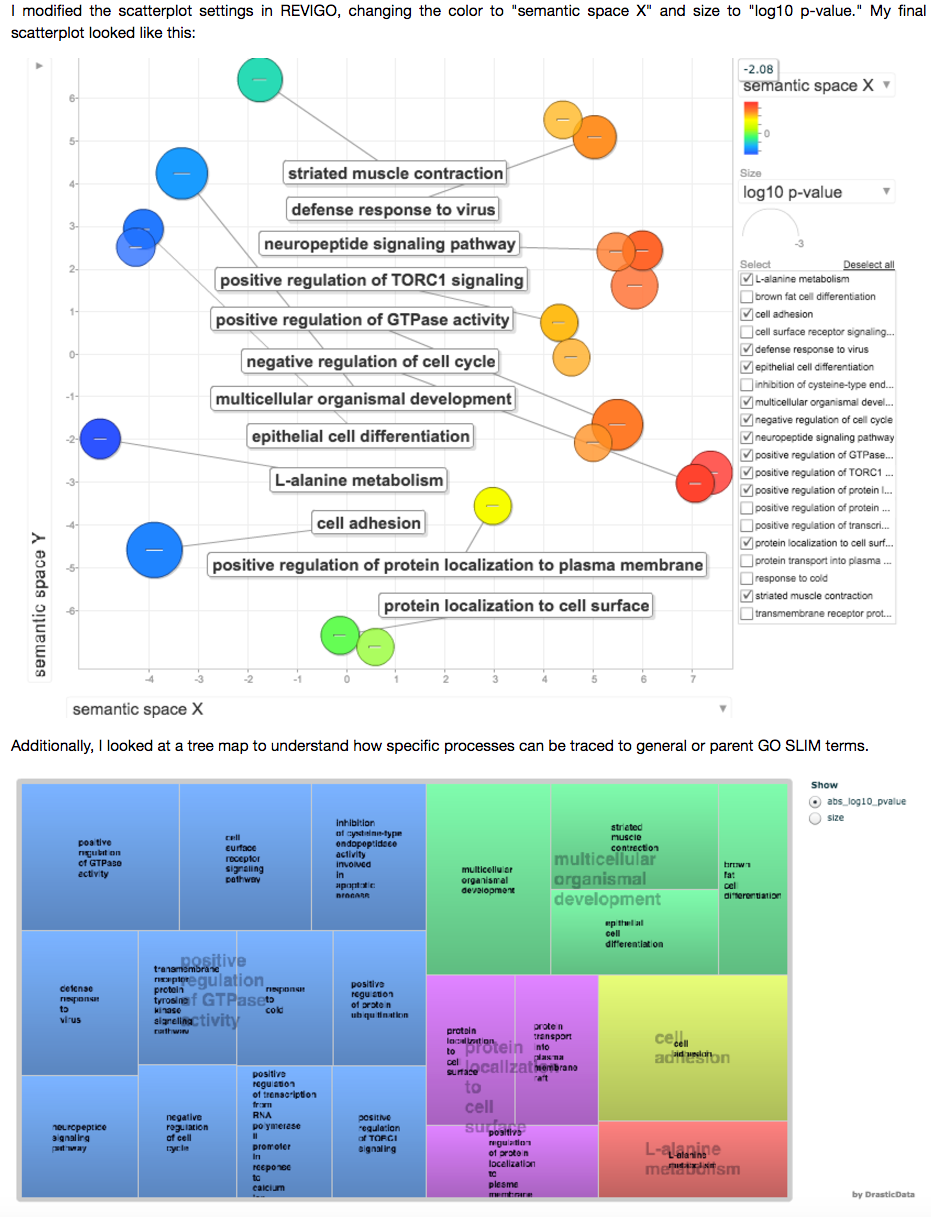
1) Identify proteins and their functions in C. gigas proteome
TAB file with protein names, GO terms, e-values, etc. [C. gigas GO terms](https://github.com/Ellior2/Fish-546-Bioinformatics/blob/master/analyses/gigas_prot/C_gigas_GOterms.tabular)
JPG with visualization from Revigo based on GO terms. [C. gigas Revigo visualization](https://github.com/Ellior2/Fish-546-Bioinformatics/blob/master/analyses/gigas_prot/C_gigas_Revigo.JPG), [Revigo CSV](https://github.com/Ellior2/Fish-546-Bioinformatics/blob/master/analyses/gigas_prot/C_gigas_REVIGO.csv)
2) Compare an oyster proteome to another bivalve- the geoduck
CSV file with table of proteins and GO terms that are shared between these two bivalve species [C. gigas and P. genorosa table](https://github.com/Ellior2/Fish-546-Bioinformatics/blob/master/analyses/gigas_prot/Cgig_Pgen_table.xlsx)
TXT files with unique proteins specific to each organism [C. gigas](https://github.com/Ellior2/Fish-546-Bioinformatics/blob/master/analyses/gigas_prot/blastoutput4.txt), [P. genorosa](https://github.com/Ellior2/Fish-546-Bioinformatics/blob/master/analyses/gigas_prot/blastoutput_pgen.txt)
JPG that visualizes the data [Venn Diagram](https://github.com/Ellior2/Fish-546-Bioinformatics/blob/master/analyses/gigas_prot/Venn_oyster_geoduck.JPG)
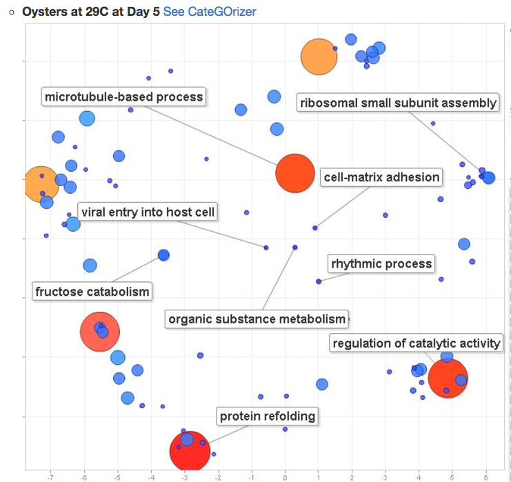
3) Draw conclusions about differential protein expression in oysters reared at 23C and 29C from 2015 MS/MS data.
TAB files listing unique proteins, their functions, and expression levels (in this case peak area) for each sample. [23C oysters at Day 5](https://github.com/Ellior2/Fish-546-Bioinformatics/blob/master/analyses/taylor/2015oyster1_23CDay5.tabular), [29C oysters at Day 5](https://github.com/Ellior2/Fish-546-Bioinformatics/blob/master/analyses/taylor/2015oyster2_29CDay5.tabular), [23C oysters at Day 8](https://github.com/Ellior2/Fish-546-Bioinformatics/blob/master/analyses/taylor/2015oyster13_23CDay8.tabular), [29C oysters at Day 8](https://github.com/Ellior2/Fish-546-Bioinformatics/blob/master/analyses/taylor/2015oyster14_29CDay8.tabular)
JPGs that visualize differences in protein expression between these two treatments
one of many….
@yaaminiv did some analysis of Ostrea lurida gonad nucleotide sequences in control and ocean acidification conditions.
Venkataraman, Yaamini (2016): Analysis of Ostrea lurida gonad nucleotide sequences in control and ocean acidification conditions. figshare. https://dx.doi.org/10.6084/m9.figshare.4339886.v1 Retrieved: 17 42, Dec 19, 2016 (GMT)
You will find a nice series of Jupyter notebooks culminating in some enrichment analyses.
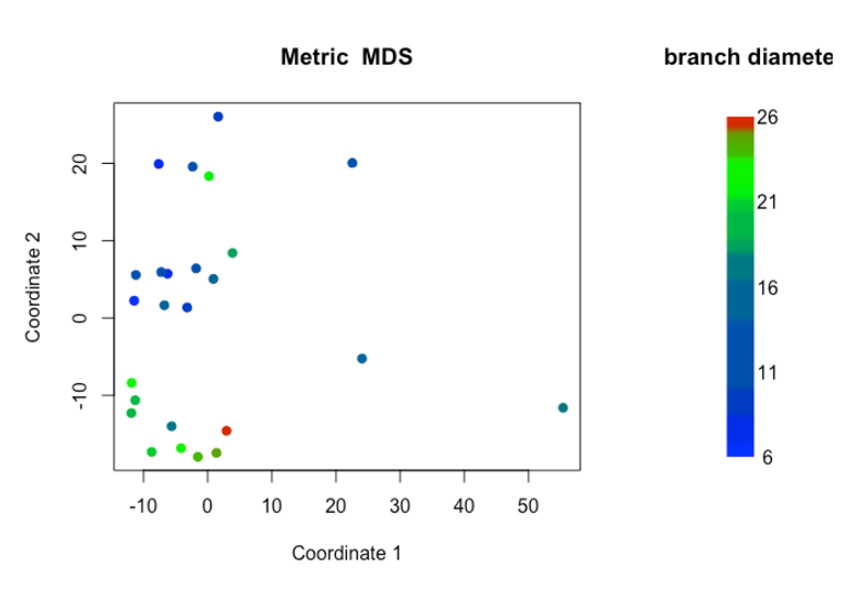
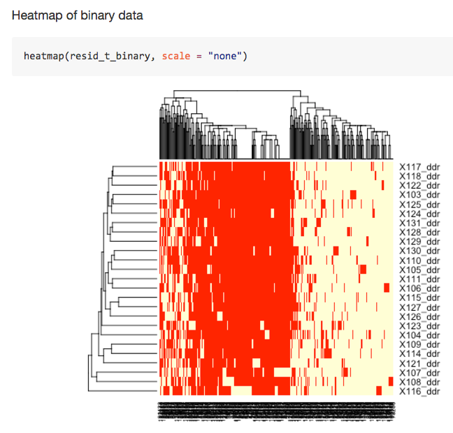
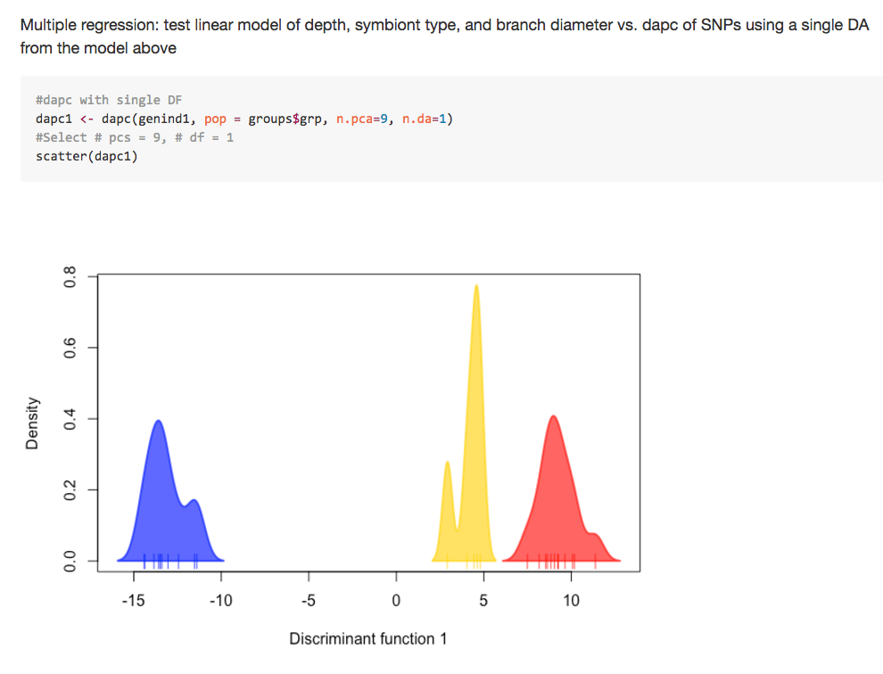
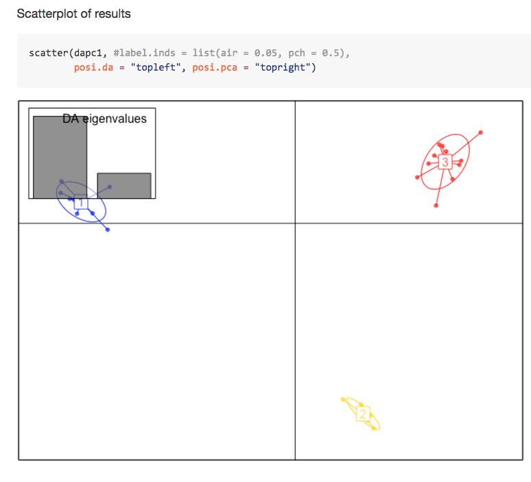
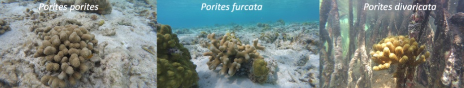
albnl @jldimond completed his project involving analysis of Porites spp. ddRAD-seq and EpiRAD-seq data.
![]()
Jay Dimond. (2016). jldimond/jldimond-fish546-2016: Porites.v2 [Data set]. Zenodo. http://doi.org/10.5281/zenodo.192371
His goal was to evaluate
(1) if there is any genetic structuring of these individuals using the ddRAD data and
(2) if there is any epigenetic structuring of these individuals using the EpiRAD data.
Check out is readme for an overview. And here are a few pics to keep you wanting more…