Navigating Annotation

The following is a stepwise example or annotation of a gene set using UniProt::Swiss-Prot (reviewed) such that Gene Ontology terms can be associated with each gene.

In this following chunk where the fasta file is downloaded the release is noted and the file name is modified accordingly.

cd misc/data

curl -O https://ftp.uniprot.org/pub/databases/uniprot/current_release/knowledgebase/complete/uniprot_sprot.fasta.gz

mv uniprot_sprot.fasta.gz uniprot_sprot_r2023_02.fasta.gz
gunzip -k uniprot_sprot_r2023_02.fasta.gz

A protein blast database is then made.

/home/shared/ncbi-blast-2.11.0+/bin/makeblastdb \
-in ../datauniprot_sprot_r2023_02.fasta \
-dbtype prot \
-out ../datauniprot_sprot_r2023_02

In a majority of cases you will want to annotate a gene set to get gene ontology information. If you are creating your own genome or transcriptome it should be rather straightforward to know what file to annotate. If using a widely studied system where there are publically available resources, it is advisable to use those as this is the best way to facilitate integration of data sets. In this case study we will be considering the Eastern oyster, (Crassostrea virginica) for which there is data at NCBI and Ensembl Metazoa. At NCBI there is both a GenBank and RefSeq assembly available.

In order to know which of the numerous fasta files should annotated with gene ontology information one should think downstream (or look to files already generated) to the identifiers in genesets that would be subject to functional enrichment tests.

The resulting fpkm count matrix for our case study is from an experiment where male and female oysters where exposed to low pH (and control) conditions. The count matrix is accessible here (csv). Hisat2/Stringtie was used to generate the count matrix with GCF_002022765.2_C_virginica-3.0_genomic.gff formatting thus responsible for gene naming. Specifically the naming format is as follows gene-LOC111099033,gene-LOC111099034,gene-LOC111099035.

The following fasta was selected for annotation: GCF_002022765.2_C_virginica-3.0_translated_cds.faa.gz

cd ../data

curl -O https://ftp.ncbi.nlm.nih.gov/genomes/all/GCF/002/022/765/GCF_002022765.2_C_virginica-3.0/GCF_002022765.2_C_virginica-3.0_translated_cds.faa.gz

gunzip -k GCF_002022765.2_C_virginica-3.0_translated_cds.faa.gz

head -2 ../data/GCF_002022765.2_C_virginica-3.0_translated_cds.faa

echo "number of sequences"
grep -c  ">" ../data/GCF_002022765.2_C_virginica-3.0_translated_cds.faa

>lcl|NC_035780.1_prot_XP_022327646.1_1 [gene=LOC111126949] [db_xref=GeneID:111126949] [protein=UNC5C-like protein] [protein_id=XP_022327646.1] [location=join(30535..31557,31736..31887,31977..32565,32959..33204)] [gbkey=CDS]
MTEVCYIWASSSTTVVICGIFFIVWRCFISIKKRASPLHGSSQQVCQTCQIEGHDFGEFQLSCRRQNTNVGYDLQGRRSD

This protein fasta is used as query for blast of uniprot_sprot database.

/home/shared/ncbi-blast-2.11.0+/bin/blastp \
-query ../data/GCF_002022765.2_C_virginica-3.0_translated_cds.faa \
-db ../data/uniprot_sprot_r2023_02 \
-out ../data/Cvir_transcds-uniprot_blastp.tab \
-evalue 1E-20 \
-num_threads 40 \
-max_target_seqs 1 \
-outfmt 6

Here is what the output file looks like, and at this point we want to get the UniProt Accession number for each gene

head -2 ../data/Cvir_transcds-uniprot_blastp.tab

## lcl|NC_035780.1_prot_XP_022327646.1_1    sp|Q8IV45|UN5CL_HUMAN   33.403  479 270 8   151 626 78  510 4.80e-77    258
## lcl|NC_035780.1_prot_XP_022305632.1_4    sp|P39021|MEOX2_XENLA   55.118  127 57  0   104 230 115 241 5.84e-38    138

blast <- read.csv("../data/Cvir_transcds-uniprot_blastp.tab", sep = '\t', header = FALSE)

Convert fasta to tab

perl -e '$count=0; $len=0; while(<>) {s/\r?\n//; s/\t/ /g; if (s/^>//) { if ($. != 1) {print "\n"} s/ |$/\t/; $count++; $_ .= "\t";} else {s/ //g; $len += length($_)} print $_;} print "\n"; warn "\nConverted $count FASTA records in $. lines to tabular format\nTotal sequence length: $len\n\n";' \
../data/GCF_002022765.2_C_virginica-3.0_translated_cds.faa > ../data/GCF_002022765.2_C_virginica-3.0_translated_cds.tab

## 
## Converted 60213 FASTA records in 580876 lines to tabular format
## Total sequence length: 39274970

head -1 ../data/GCF_002022765.2_C_virginica-3.0_translated_cds.tab

## lcl|NC_035780.1_prot_XP_022327646.1_1    [gene=LOC111126949] [db_xref=GeneID:111126949] [protein=UNC5C-like protein] [protein_id=XP_022327646.1] [location=join(30535..31557,31736..31887,31977..32565,32959..33204)] [gbkey=CDS]    MTEVCYIWASSSTTVVICGIFFIVWRCFISIKKRASPLHGSSQQVCQTCQIEGHDFGEFQLSCRRQNTNVGYDLQGRRSDVTAIIQGQSVLRPSPVPVEVLPVEGNRVSRTSESVRTHSSTHSAGSSSHVATSPVMSSCSVGKETSLNPYSYCRDIYSISERSTMKTVGGKLVVSVAHYVTSRGDWLMLDDMGISLRIPPNAVPVGEEKLICLVLNWDLGDNPPMTGTDSLVSPVVFVGPHGLKLNKPCELHYRHCAYDPRQIVVLRSETDLHGDKHWTEMCGQENQDGVCRLSSDECILQIDTFTLYTCIQRPLRNLKMAKWLQIAAFSNPLEKRIDHHEVRVYFLNKTPCALQWAIQNEAQFQHVLICPEKAFLFHGQVDDILDIRVTLKYLSADWESIDNDVYERVPYLHIWHGQCPHIVMCFKKKPKHSVRELNFHLNIYQDTLENEGEKIVVHATENPRCVYDNSCIINIHTSDSPEKKTLPNVEVKKTEDNVNVSIKQSHSPSAALLEEMRTESTQYIPYDIRKHLKVKLDPPNPLGNDWRRLAEVLDLSQFIEYLKSLHSSPTETLLSVIEHRNISLEELATMLNEIQRYDAEKIVSDYLHQHQNSSPVCIRGGLQHDERPFAHMSATNNLSNVEPDNVSQEENRAQYLPLGNSGHDNNAYM

cdsftab <- read.csv("../data/GCF_002022765.2_C_virginica-3.0_translated_cds.tab", sep = '\t', header = FALSE, row.names=NULL)

Now we can take the two data frames: A) blast output of taking protein fasta and comparing to uniprot_swiss-prot and B) a tabular version of same fasta file that has ID numbers of importance. Note this importance was determined based on what we want to use down stream.

g.spid <- left_join(blast, cdsftab, by = "V1") %>%
  mutate(gene = str_extract(V2.y, "(?<=\\[gene=)\\w+")) %>%
  select(gene, V11, V2.x) %>%
  mutate(SPID = str_extract(V2.x, "(?<=\\|)[^\\|]*(?=\\|)")) %>%
  distinct(gene, SPID, .keep_all = TRUE)

Let’s break it down step by step:

g.spid <- left_join(blast, cdsftab, by = "V1") - This line is using the left_join() function from dplyr to merge the blast and cdsftab datasets by the column “V1”. A left join retains all the rows in the blast data frame and appends the matching rows in the cdsftab data frame. If there is no match, the result is NA. The result of this operation is assigned to the g.spid object.
mutate(gene = str_extract(V2.y, "(?<=\\[gene=)\\w+")) - This line is using the mutate() function from dplyr to add a new column called “gene” to the data frame. The new column is created by extracting substrings from the “V2.y” column based on the given regular expression pattern "(?<=\\[gene=)\\w+". This regular expression matches and extracts any word (sequence of word characters, i.e., alphanumeric and underscore) that comes after “[gene=”.
select(gene, V11, V2.x) - This line is using the select() function from dplyr to keep only the specified columns (“gene”, “V11”, and “V2.x”) in the data frame.
mutate(SPID = str_extract(V2.x, "(?<=\\|)[^\\|]*(?=\\|)")) - Again, the mutate() function is used to add another new column named “SPID”. This column is created by extracting substrings from the “V2.x” column. The regular expression "(?<=\\|)[^\\|]*(?=\\|)" is designed to extract any character(s) that is/are surrounded by “|” (pipe symbol). This is a common format for delimited strings.
distinct(gene, SPID, .keep_all = TRUE) - This line is using the distinct() function from dplyr to remove duplicate rows based on the “gene” and “SPID” columns. The .keep_all = TRUE argument means that all other columns are also kept in the result, not just the “gene” and “SPID” columns.

The resulting g.spid data frame should have unique rows with respect to the “gene” and “SPID” columns, and it should contain these two new columns, “gene” and “SPID”, extracted from the original data based on specific string patterns.

Now lets just write out SPIDs.

left_join(blast, cdsftab, by = "V1") %>%
  mutate(gene = str_extract(V2.y, "(?<=\\[gene=)\\w+")) %>%
  select(gene, V11, V2.x) %>%
  mutate(SPID = str_extract(V2.x, "(?<=\\|)[^\\|]*(?=\\|)")) %>%
  distinct(gene, SPID, .keep_all = TRUE) %>%
  select(SPID) %>%
  write.table(file = "../data/SPID.txt", sep = "\t", row.names = FALSE, quote = FALSE
 ) 

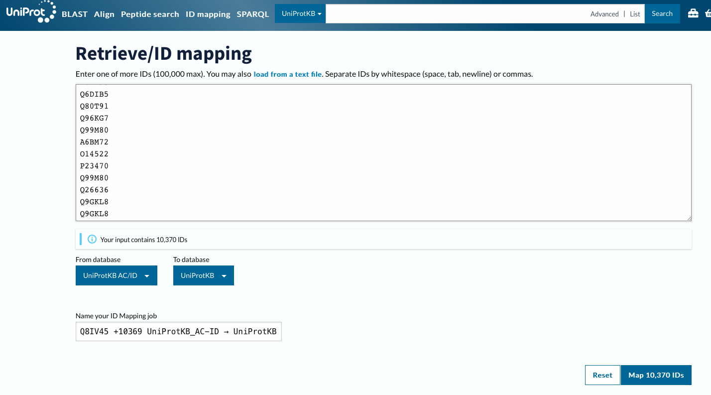
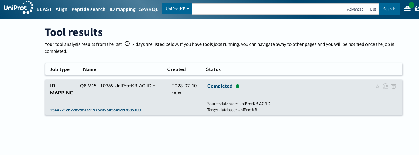
With a list of matching Swiss-Prot IDs, (technically UniProt Accession number) we can go back to https://www.uniprot.org and grab corresponding GO terms. This can be done via a web or using Python API.

Using Web

Using ID Mapping

Now will customize columns to get GO IDs.

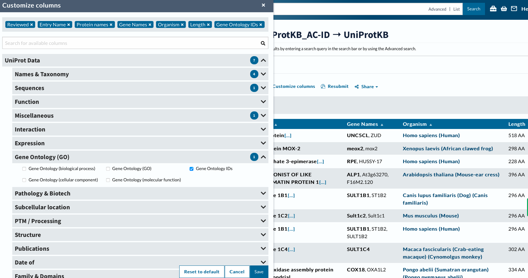
head -2 ../data/uniprotGO.tab

## From Entry   Reviewed    Entry Name  Protein names   Gene Names  Organism    Length  Gene Ontology IDs
## Q8IV45   Q8IV45  reviewed    UN5CL_HUMAN UNC5C-like protein (Protein unc-5 homolog C-like) (ZU5 and death domain-containing protein) UNC5CL ZUD  Homo sapiens (Human)    518 GO:0005042; GO:0005737; GO:0008233; GO:0016020; GO:0043123; GO:0046330

Finally we can join table to get “LOCIDs” the notation for our DEGs, with GO terms.

go <- read.csv("../data/uniprotGO.tab", sep = '\t', header = TRUE, row.names=NULL)

left_join(g.spid, go, by = c("SPID" = "Entry")) %>%
  select(gene,Gene.Ontology.IDs) %>%
  write.table(file = "../data/geneGO.txt", sep = "\t", row.names = FALSE, quote = FALSE
  )

head ../data/geneGO.txt

## gene Gene.Ontology.IDs
## LOC111126949 GO:0005042; GO:0005737; GO:0008233; GO:0016020; GO:0043123; GO:0046330
## LOC111112434 GO:0000981; GO:0003700; GO:0005634; GO:0016607; GO:0043565; GO:0045944
## LOC111120752 GO:0004750; GO:0005829; GO:0005975; GO:0006098; GO:0009052; GO:0042802; GO:0042803; GO:0046872; GO:0070062
## LOC111105685 GO:0003682; GO:0004518; GO:0005634; GO:0035098; GO:0035102; GO:0040029; GO:0046872
## LOC111113860 GO:0004062; GO:0005737; GO:0006068; GO:0006805; GO:0008146; GO:0009812; GO:0030855; GO:0042403; GO:0050427; GO:0051923
## LOC111109550 GO:0004062; GO:0005737; GO:0005764; GO:0008146; GO:0051923
## LOC111109753 GO:0004062; GO:0005737; GO:0005829; GO:0006068; GO:0006576; GO:0006805; GO:0008146; GO:0009812; GO:0018958; GO:0030855; GO:0042403; GO:0050427; GO:0051923
## LOC111109452 GO:0004062; GO:0005829; GO:0008146; GO:0009812; GO:0050427
## LOC111101273 GO:0005743; GO:0008535; GO:0032977; GO:0032979; GO:0033617; GO:0051204

Written on July 8, 2023