
Revisiting EpiDiverse SNPs
Steven Roberts 24 July, 2023
Sam ran Epidiverse
https://github.com/sr320/ceabigr/issues/69#issuecomment-1258238481
- Notebook
- VCF Directory - https://gannet.fish.washington.edu/Atumefaciens/20220921-cvir-ceabigr-nextflow-epidiverse-snp/snps/vcf/
- results dir - https://gannet.fish.washington.edu/Atumefaciens/20220921-cvir-ceabigr-nextflow-epidiverse-snp/snps/stats/
0.1 Merging Epidiverse VCFs
Next step for capturing SNP info in Epidiverse Workflow is merging.
cd ../data/big
wget -r \
--no-directories --no-parent \
-P . \
-A "*vcf.g*" https://gannet.fish.washington.edu/Atumefaciens/20220921-cvir-ceabigr-nextflow-epidiverse-snp/snps/vcf/
/home/shared/bcftools-1.14/bcftools  merge \
--force-samples \
../data/big/*.vcf.gz \
--merge all \
--threads 40 \
-O v \
-o ../output/51-SNPs/EpiDiv_merged.vcf
head -20 ../output/51-SNPs/EpiDiv_merged.vcf## ##fileformat=VCFv4.2
## ##FILTER=<ID=PASS,Description="All filters passed">
## ##fileDate=20220924
## ##source=freeBayes v1.3.2-dirty
## ##reference=GCF_002022765.2_C_virginica-3.0_genomic.fa
## ##contig=<ID=NC_035780.1,length=65668440>
## ##contig=<ID=NC_035781.1,length=61752955>
## ##contig=<ID=NC_035782.1,length=77061148>
## ##contig=<ID=NC_035783.1,length=59691872>
## ##contig=<ID=NC_035784.1,length=98698416>
## ##contig=<ID=NC_035785.1,length=51258098>
## ##contig=<ID=NC_035786.1,length=57830854>
## ##contig=<ID=NC_035787.1,length=75944018>
## ##contig=<ID=NC_035788.1,length=104168038>
## ##contig=<ID=NC_035789.1,length=32650045>
## ##contig=<ID=NC_007175.2,length=17244>
## ##phasing=none
## ##commandline="freebayes -f GCF_002022765.2_C_virginica-3.0_genomic.fa 12M_R1_val_1_bismark_bt2_pe.deduplicated.sorted.bam --strict-vcf --no-partial-observations --report-genotype-likelihood-max --genotype-qualities --min-repeat-entropy 1 --min-coverage 0 --min-base-quality 1 --region NC_035780.1:0-100000"
## ##INFO=<ID=NS,Number=1,Type=Integer,Description="Number of samples with data">
## ##INFO=<ID=DP,Number=1,Type=Integer,Description="Total read depth at the locus">The eventual GRM does not have sample names so wanted to check order of merged files (assuming this is related to how GRM file is created)
fgrep "R1_val_1" ../output/51-SNPs/EpiDiv_merged.vcf##commandline="freebayes -f GCF_002022765.2_C_virginica-3.0_genomic.fa 12M_R1_val_1_bismark_bt2_pe.deduplicated.sorted.bam --strict-vcf --no-partial-observations --report-genotype-likelihood-max --genotype-qualities --min-repeat-entropy 1 --min-coverage 0 --min-base-quality 1 --region NC_035780.1:0-100000"
##bcftools_viewCommand=view -Oz 12M_R1_val_1_bismark_bt2_pe.deduplicated.sorted.vcf; Date=Sat Sep 24 13:39:51 2022
##bcftools_mergeCommand=merge --force-samples --merge all --threads 40 -O v -o ../output/51-SNPs/EpiDiv_merged.vcf ../data/big/12M_R1_val_1_bismark_bt2_pe.deduplicated.sorted.vcf.gz ../data/big/13M_R1_val_1_bismark_bt2_pe.deduplicated.sorted.vcf.gz ../data/big/16F_R1_val_1_bismark_bt2_pe.deduplicated.sorted.vcf.gz ../data/big/19F_R1_val_1_bismark_bt2_pe.deduplicated.sorted.vcf.gz ../data/big/22F_R1_val_1_bismark_bt2_pe.deduplicated.sorted.vcf.gz ../data/big/23M_R1_val_1_bismark_bt2_pe.deduplicated.sorted.vcf.gz ../data/big/29F_R1_val_1_bismark_bt2_pe.deduplicated.sorted.vcf.gz ../data/big/31M_R1_val_1_bismark_bt2_pe.deduplicated.sorted.vcf.gz ../data/big/35F_R1_val_1_bismark_bt2_pe.deduplicated.sorted.vcf.gz ../data/big/36F_R1_val_1_bismark_bt2_pe.deduplicated.sorted.vcf.gz ../data/big/39F_R1_val_1_bismark_bt2_pe.deduplicated.sorted.vcf.gz ../data/big/3F_R1_val_1_bismark_bt2_pe.deduplicated.sorted.vcf.gz ../data/big/41F_R1_val_1_bismark_bt2_pe.deduplicated.sorted.vcf.gz ../data/big/44F_R1_val_1_bismark_bt2_pe.deduplicated.sorted.vcf.gz ../data/big/48M_R1_val_1_bismark_bt2_pe.deduplicated.sorted.vcf.gz ../data/big/50F_R1_val_1_bismark_bt2_pe.deduplicated.sorted.vcf.gz ../data/big/52F_R1_val_1_bismark_bt2_pe.deduplicated.sorted.vcf.gz ../data/big/53F_R1_val_1_bismark_bt2_pe.deduplicated.sorted.vcf.gz ../data/big/54F_R1_val_1_bismark_bt2_pe.deduplicated.sorted.vcf.gz ../data/big/59M_R1_val_1_bismark_bt2_pe.deduplicated.sorted.vcf.gz ../data/big/64M_R1_val_1_bismark_bt2_pe.deduplicated.sorted.vcf.gz ../data/big/6M_R1_val_1_bismark_bt2_pe.deduplicated.sorted.vcf.gz ../data/big/76F_R1_val_1_bismark_bt2_pe.deduplicated.sorted.vcf.gz ../data/big/77F_R1_val_1_bismark_bt2_pe.deduplicated.sorted.vcf.gz ../data/big/7M_R1_val_1_bismark_bt2_pe.deduplicated.sorted.vcf.gz ../data/big/9M_R1_val_1_bismark_bt2_pe.deduplicated.sorted.vcf.gz; Date=Sun May 7 10:33:42 2023Here is the filtering steps
Let’s break down the command:
/home/shared/vcftools-0.1.16/bin/vcftools: This is the path to the VCFtools program. You’re executing the program from its location.--vcf ../output/51-SNPs/EpiDiv_merged.vcf: This specifies the input VCF file that you’re going to work with.--recode --recode-INFO-all: The--recodeoption tells VCFtools to generate a new VCF file as output after performing all of the filtering operations. The--recode-INFO-alltells VCFtools to keep all INFO fields from the input VCF in the new output file.--min-alleles 2 --max-alleles 2: This filters the data to include only bi-allelic sites, meaning sites that have exactly two alleles (one could be the reference allele, and the other is the variant allele).--max-missing 0.5: This is a filter that sets a maximum allowable proportion of individuals with missing data at each site. In this case, it discards any variants where more than 50% of the data is missing.--mac 2: This option tells the program to only include sites with a Minor Allele Count of at least 2. This means that the less common variant must appear at least twice in your sample.--out ../output/51-SNPs/EpiDiv_merged.f: This is the location and prefix of the output files. Several files might be generated depending on the options you used, and they’ll all start with this prefix.
So, in summary, this command is running a filtering process on a VCF file, and then saving a new VCF file that only includes bi-allelic sites (those with exactly 2 alleles) where less than 50% of the data is missing and the less common variant appears at least twice. The new file will keep all the INFO fields from the original VCF.
/home/shared/vcftools-0.1.16/bin/vcftools \
--vcf ../output/51-SNPs/EpiDiv_merged.vcf \
--recode --recode-INFO-all \
--min-alleles 2 --max-alleles 2 \
--max-missing 0.5 \
--mac 2 \
--out ../output/51-SNPs/EpiDiv_merged.f.recode.vcf
After filtering, kept 26 out of 26 Individuals Outputting VCF file… After filtering, kept 2343637 out of a possible 144873997 Sites Run Time = 897.00 seconds
head -20 ../output/51-SNPs/EpiDiv_merged.f.recode.vcf## ##fileformat=VCFv4.2
## ##FILTER=<ID=PASS,Description="All filters passed">
## ##fileDate=20220924
## ##source=freeBayes v1.3.2-dirty
## ##reference=GCF_002022765.2_C_virginica-3.0_genomic.fa
## ##contig=<ID=NC_035780.1,length=65668440>
## ##contig=<ID=NC_035781.1,length=61752955>
## ##contig=<ID=NC_035782.1,length=77061148>
## ##contig=<ID=NC_035783.1,length=59691872>
## ##contig=<ID=NC_035784.1,length=98698416>
## ##contig=<ID=NC_035785.1,length=51258098>
## ##contig=<ID=NC_035786.1,length=57830854>
## ##contig=<ID=NC_035787.1,length=75944018>
## ##contig=<ID=NC_035788.1,length=104168038>
## ##contig=<ID=NC_035789.1,length=32650045>
## ##contig=<ID=NC_007175.2,length=17244>
## ##phasing=none
## ##commandline="freebayes -f GCF_002022765.2_C_virginica-3.0_genomic.fa 12M_R1_val_1_bismark_bt2_pe.deduplicated.sorted.bam --strict-vcf --no-partial-observations --report-genotype-likelihood-max --genotype-qualities --min-repeat-entropy 1 --min-coverage 0 --min-base-quality 1 --region NC_035780.1:0-100000"
## ##INFO=<ID=NS,Number=1,Type=Integer,Description="Number of samples with data">
## ##INFO=<ID=DP,Number=1,Type=Integer,Description="Total read depth at the locus">fgrep "R1_val_1" ../output/51-SNPs/EpiDiv_merged.f.recode.vcf1 NgsRelate
a la
https://github.com/RobertsLab/resources/issues/1681#issuecomment-1642557685
chatGPT
First, let’s understand what these tools are.
ngsRelate: This is a software package used for inferring pairwise relatedness from next-generation sequencing (NGS) data. It can calculate different coefficients of relatedness as well as inbreeding coefficients.
spaa: This is an R package that can calculate the genomic relationship matrix (GRM) and genomic kinship matrix (GKM) using SNP array and NGS data.
As of version 2, NgsRelate can parse BCF/VCF files using htslib with the following command:
./ngsrelate  -h my.VCF.gz -O vcf.res
By default, NgsRelate will estimate the allele frequencies using the individuals provided in the VCF files. Allele frequencies from the INFO field can used be used instead using -A TAG. The TAG usually take the form of AF or AF1 but can be set to anything. By default the PL data (Phred-scaled likelihoods for genotypes) is parsed, however, the called genotypes can also be used instead with the -T GT option. If called genotypes are being used, the software requires an additional argument (-c 1). If using -c 2, ngsRelate calls genotypes assuming hardy-weinberg.
cut -d ',' -f 1 <<EOF
12M,S12M,Exposed,M,3,EM05
13M,S13M,Control,M,1,CM04
16F,S16F,Control,F,2,CF05
19F,S19F,Control,F,2,CF08
22F,S22F,Exposed,F,4,EF02
23M,S23M,Exposed,M,3,EM04
29F,S29F,Exposed,F,4,EF07
31M,S31M,Exposed,M,3,EM06
35F,S35F,Exposed,F,4,EF08
36F,S36F,Exposed,F,4,EF05
39F,S39F,Control,F,2,CF06
3F,S3F,Exposed,F,4,EF06
41F,S41F,Exposed,F,4,EF03
44F,S44F,Control,F,2,CF03
48M,S48M,Exposed,M,3,EM03
50F,S50F,Exposed,F,4,EF01
52F,S52F,Control,F,2,CF07
53F,S53F,Control,F,2,CF02
54F,S54F,Control,F,2,CF01
59M,S59M,Exposed,M,3,EM01
64M,S64M,Control,M,1,CM05
6M,S6M,Control,M,1,CM02
76F,S76F,Control,F,2,CF04
77F,S77F,Exposed,F,4,EF04
7M,S7M,Control,M,1,CM01
9M,S9M,Exposed,M,3,EM02
EOF/home/shared/ngsRelate/ngsRelate/ngsRelate \
-h ../output/51-SNPs/EpiDiv_merged.f.recode.vcf \
-T GT \
-c 1 \
-z ../output/53-revisit-epi-SNPs/sample.txt \
-O ../output/53-revisit-epi-SNPs/vcf.relatednesshead -2 ../output/53-revisit-epi-SNPs/vcf.relatedness## a b ida idb nSites J9 J8 J7 J6 J5 J4 J3 J2 J1 rab Fa Fb theta inbred_relatedness_1_2 inbred_relatedness_2_1 fraternity identity zygosity 2of3_IDB F_diff_a_b loglh nIter bestoptimll coverage 2dsfs R0 R1 KING 2dsfs_loglike 2dsfsf_niter
## 0 1 12M 13M 1038400 0.799793 0.000003 0.051831 0.000002 0.000000 0.000000 0.000000 0.148370 0.000000 0.051833 0.148370 0.148372 0.025916 0.000000 0.000000 0.200201 0.000000 0.200201 0.200204 -0.000001 -1663336.404155 134 -1 0.493654 6.306127e-02,2.031383e-02,6.122145e-02,2.076443e-02,1.558777e-01,1.402793e-01,5.729257e-02,1.300012e-01,3.511883e-01 0.760301 0.362614 -0.130234 -1948248.937260 101.1 Output format
a  b  nSites  J9        J8        J7        J6        J5        J4        J3        J2        J1        rab       Fa        Fb        theta     inbred_relatedness_1_2  inbred_relatedness_2_1  fraternity  identity  zygosity  2of3IDB   FDiff      loglh           nIter  coverage  2dsfs                                                                             R0        R1        KING       2dsfs_loglike   2dsfsf_niter
0  1  99927   0.384487  0.360978  0.001416  0.178610  0.071681  0.000617  0.002172  0.000034  0.000005  0.237300  0.002828  0.250330  0.127884  0.001091                0.035846                0.001451    0.000005  0.001456  0.345411  -0.088997  -341223.335664  103    0.999270  0.154920,0.087526,0.038724,0.143087,0.155155,0.139345,0.038473,0.087632,0.155138  0.497548  0.290124  0.000991   -356967.175857  7
The first two columns contain indices of the two individuals used for the analysis. The third column is the number of genomic sites considered. The following nine columns are the maximum likelihood (ML) estimates of the nine jacquard coefficients, where K0==J9; K1==J8; K2==J7 in absence of inbreeding. Based on these Jacquard coefficients, NgsRelate calculates 11 summary statistics:
rab is the pairwise relatedness
(J1+J7+0.75*(J3+J5)+.5*J8)Hedrick et alFa is the inbreeding coefficient of individual a
J1+J2+J3+J4JacquardFb is the inbreeding coefficient of individual b
J1+J2+J5+J6Jacquardtheta is the coefficient of kinship
J1 + 0.5*(J3+J5+J7) + 0.25*J8)Jacquardinbred_relatedness_1_2
J1+0.5*J3Ackerman et alinbred_relatedness_2_1
J1+0.5*J5Ackerman et alfraternity
J2+J7Ackerman et alidentity
J1Ackerman et alzygosity
J1+J2+J7Ackerman et alTwo-out-of-three IBD
J1+J2+J3+J5+J7+0.5*(J4+J6+J8)Miklos csurosInbreeding difference
0.5*(J4-J6)Miklos csurosthe log-likelihood of the ML estimate.
number of EM iterations. If a
-1is displayed. A boundary estimate had a higher likelihood.If differs from
-1, a boundary estimate had a higher likelihood. Reported loglikelihood should be highly similar to the corresponding value reported inloglhfraction of sites used for the ML estimate
The remaining columns relate to statistics based on a 2D-SFS.
2dsfs estimates using the same methodology as implemented in realSFS, see ANGSD
R0 Waples et al
R1 Waples et al
KING Waples et al
the log-likelihood of the 2dsfs estimate.
number of iterations for 2dsfs estimate
You can also input a file with the IDs of the individuals (on ID per line), using the -z option, in the same order as in the file filelist used to make the genotype likelihoods or the VCF file. If you do the output will also contain these IDs as column 3 and 4.
Note that in some cases nIter is -1. This indicates that values on the boundary of the parameter space had a higher likelihood than the values achieved using the EM-algorithm (ML methods sometimes have trouble finding the ML estimate when it is on the boundary of the parameter space, and we therefore test the boundary values explicitly and output these if these have the highest likelihood)
df = read.table("../output/53-revisit-epi-SNPs/vcf.relatedness",header = T)
dfrab <- df[,c("ida","idb","rab")]
distrab <- as.matrix(list2dist(dfrab))

write.table(distrab,file="../output/53-revisit-epi-SNPs/epiMATRIX_mbd_rab.txt", col.names = T, row.names = T, sep = "\t")
# Plot the heatmap
heatmap(distrab, Rowv = NA, Colv = NA, col = cm.colors(256), scale = "none")
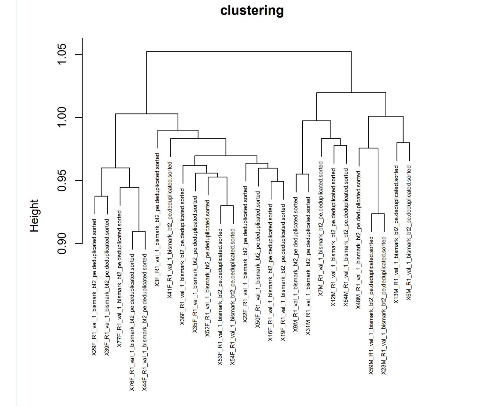
# Perform hierarchical clustering
hc <- hclust(dist(distrab))

# Plot the dendrogram (cladogram)
plot(hc, hang = -1, main = "Cladogram")

# If you want to add labels to the leaves of the tree (optional):
labels <- rownames(distrab)
rect.hclust(hc, k = 6, border = "gray")
Citation
@online{roberts2023,
  author = {Roberts, Steven},
  title = {Epidiverse {GRM}},
  date = {2023-07-24},
  url = {https://sr320.github.io/tumbling-oysters/posts/sr320-03-grm/},
  langid = {en}
}